Assessing Read Quality, Trimming and Filtering
Overview
Teaching: 45 min
Exercises: 45 minQuestions
How can I describe the quality of my data?
How can we get rid of sequence data that doesn’t meet our quality standards?
How do these methods differ when looking at Nanopore data?
Objectives
Interpret a FastQC plot summarizing per-base quality across all reads.
Interpret the NanoPlot output summarizing a Nanopore sequencing run
Filter Nanopore reads based on quality using the command line tool SeqKit
Getting started
The first thing we need to do is log in to our cloud instance.
-
Open the cloudspan folder you created for the course
Open your file manager and navigate to the
cloudspanfolder (hint: we recommended you make the folder in your Desktop directory - but you might have made it somewhere else). If you cannot find the folder, you can remind yourself where it is stored by looking at the absolute path you wrote down in the previous episode.The folder should contain the login key file we downloaded in the previous episode and nothing else.
-
Right-click and open your machine’s command line interface
Now we can open the command line.
For Windows users:
- Right click anywhere inside the blank space of the file manager, then select Git Bash Here.
For Mac users:
You have two options.
EITHER
- Open Terminal in one window and type
cdfollowed by a space. Do not press enter! Now open Finder in another window. Drag and drop thecloudspanfolder from the Finder to the Terminal. You should see the file path leading to yourcloudspanfolder appear. Now press enter to navigate to the folder.
OR
- Open Terminal and type
cdfollowed by the absolute path that leads to yourcloudspanfolder. Press enter.
-
Login into your instance
$ ssh -i login-key-instanceNNN.pem csuser@instanceNNN.cloud-span.aws.york.ac.uk
Be sure to replace NNN with your own number, twice.
Reminder: our file structure
Before we start, here’s a reminder of what our file structure looks like as a hierarchy tree:
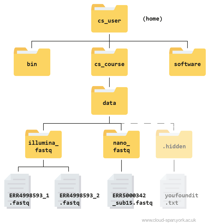 Keep this in mind as we continue to navigate the file system, and don’t hesitate to refer back to it if needed.
Quality control
Before assembling our metagenome from the the short-read Illumina sequences and the long-read Nanopore sequences, we need to apply quality control to both. The two types of sequence data require different QC methods. We will use:
- FastQC to examine the quality of the short-read Illumina data
- NanoPlot to examine the quality of the long-read Nanopore data and Seqkit to trim and filter them.
Illumina Quality control using FastQC
In previous lessons we had a look at our data files and found they were in FASTQ format, a common format for sequencing data. We used grep to look for ‘bad reads’ containing more than three consecutive Ns and put these reads into their own text file.
This could be rather time consuming and is very nuanced. Luckily, there’s a better way! Rather than assessing every read in the raw data by hand we can use FastQC to visualise the quality of the whole sequencing file.
About FastQC
Rather than looking at quality scores for each individual read, FastQC looks at quality collectively across all reads within a sample. The image below shows one FastQC-generated plot that indicates a very high quality sample:
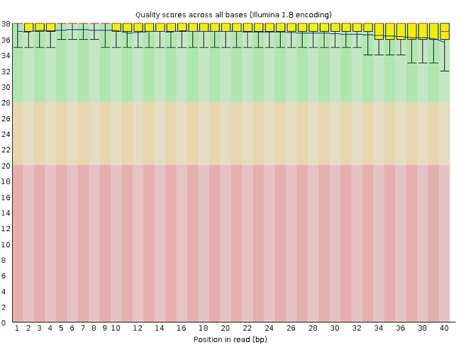
The x-axis displays the base position (bp) in the read, and the y-axis shows quality scores. In this example, the sample contains reads that are 40 bp long.
Each position has a box-and-whisker plot showing the distribution of quality scores for all reads at that position.
- The horizontal red line indicates the median quality score.
- The yellow box shows the 1st to 3rd quartile range (this means that 50% of reads have a quality score that falls within the range of the yellow box at that position).
- The whiskers show the absolute range, which covers the lowest (0th quartile) to highest (4th quartile) values.
- The plot background is also color-coded to identify good (green), acceptable (yellow), and bad (red) quality scores.
Now let’s take a look at a quality plot on the other end of the spectrum.
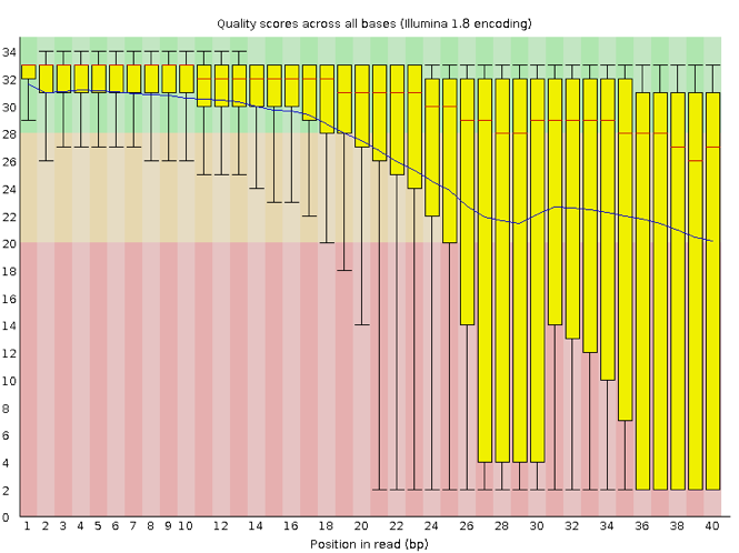
Here, we see positions within the read in which the boxes span a much wider range. Also, quality scores drop quite low into the “bad” range, particularly on the tail end of the reads. The FastQC tool produces several other diagnostic plots to assess sample quality, in addition to the one plotted above.
Getting started with FastQC
First, we are going to organise our analysis by creating a directory to contain the output of all of the analysis we generate in this course.
The mkdir command can be used to make a new directory. Using the -p flag for mkdir allows it to create a new directory, even if one of the parent directories doesn’t already exist. It also suppresses errors if the directory already exists, without overwriting that directory.
Return to your home directory (/home/csuser)
cd
Create the directories analysis/qc/illumina_qc inside cs_course
mkdir -p cs_course/analysis/qc/illumina_qc
You might want to use ls to check those nested directories have been made.
Now we have created the directories we are ready to start the quality control of the Illumina data.
FastQC has been installed on your instance and we can run it with the -h flag to display the help documentation and remind ourselves how to use it and all the parameters available:
$ fastqc -h
FastQC seq help documentation
            FastQC - A high throughput sequence QC analysis tool

SYNOPSIS

      fastqc seqfile1 seqfile2 .. seqfileN

    fastqc [-o output dir] [--(no)extract] [-f fastq|bam|sam]
           [-c contaminant file] seqfile1 .. seqfileN

DESCRIPTION

    FastQC reads a set of sequence files and produces from each one a quality
    control report consisting of a number of different modules, each one of
    which will help to identify a different potential type of problem in your
    data.

    If no files to process are specified on the command line then the program
    will start as an interactive graphical application.  If files are provided
    on the command line then the program will run with no user interaction
    required.  In this mode it is suitable for inclusion into a standardised
    analysis pipeline.

    The options for the program as as follows:

    -h --help       Print this help file and exit

    -v --version    Print the version of the program and exit

    -o --outdir     Create all output files in the specified output directory.
                    Please note that this directory must exist as the program
                    will not create it.  If this option is not set then the
                    output file for each sequence file is created in the same
                    directory as the sequence file which was processed.

    --casava        Files come from raw casava output. Files in the same sample
                    group (differing only by the group number) will be analysed
                    as a set rather than individually. Sequences with the filter
                    flag set in the header will be excluded from the analysis.
                    Files must have the same names given to them by casava
                    (including being gzipped and ending with .gz) otherwise they
                    won't be grouped together correctly.

    --nano          Files come from nanopore sequences and are in fast5 format. In
                    this mode you can pass in directories to process and the program
                    will take in all fast5 files within those directories and produce
                    a single output file from the sequences found in all files.

    --nofilter      If running with --casava then don't remove read flagged by
                    casava as poor quality when performing the QC analysis.

    --extract       If set then the zipped output file will be uncompressed in
                    the same directory after it has been created.  By default
                    this option will be set if fastqc is run in non-interactive
                    mode.

    -j --java       Provides the full path to the java binary you want to use to
                    launch fastqc. If not supplied then java is assumed to be in
                    your path.

    --noextract     Do not uncompress the output file after creating it.  You
                    should set this option if you do not wish to uncompress
                    the output when running in non-interactive mode.

    --nogroup       Disable grouping of bases for reads >50bp. All reports will
                    show data for every base in the read.  WARNING: Using this
                    option will cause fastqc to crash and burn if you use it on
                    really long reads, and your plots may end up a ridiculous size.
                    You have been warned!

    --min_length    Sets an artificial lower limit on the length of the sequence
                    to be shown in the report.  As long as you set this to a value
                    greater or equal to your longest read length then this will be
                    the sequence length used to create your read groups.  This can
                    be useful for making directly comaparable statistics from
                    datasets with somewhat variable read lengths.

    -f --format     Bypasses the normal sequence file format detection and
                    forces the program to use the specified format.  Valid
                    formats are bam,sam,bam_mapped,sam_mapped and fastq

    -t --threads    Specifies the number of files which can be processed
                    simultaneously.  Each thread will be allocated 250MB of
                    memory so you shouldn't run more threads than your
                    available memory will cope with, and not more than
                    6 threads on a 32 bit machine

    -c              Specifies a non-default file which contains the list of
    --contaminants  contaminants to screen overrepresented sequences against.
                    The file must contain sets of named contaminants in the
                    form name[tab]sequence.  Lines prefixed with a hash will
                    be ignored.

    -a              Specifies a non-default file which contains the list of
    --adapters      adapter sequences which will be explicity searched against
                    the library. The file must contain sets of named adapters
                    in the form name[tab]sequence.  Lines prefixed with a hash
                    will be ignored.

    -l              Specifies a non-default file which contains a set of criteria
    --limits        which will be used to determine the warn/error limits for the
                    various modules.  This file can also be used to selectively
                    remove some modules from the output all together.  The format
                    needs to mirror the default limits.txt file found in the
                    Configuration folder.

   -k --kmers       Specifies the length of Kmer to look for in the Kmer content
                    module. Specified Kmer length must be between 2 and 10. Default
                    length is 7 if not specified.

   -q --quiet       Supress all progress messages on stdout and only report errors.

   -d --dir         Selects a directory to be used for temporary files written when
                    generating report images. Defaults to system temp directory if
                    not specified.

BUGS

    Any bugs in fastqc should be reported either to simon.andrews@babraham.ac.uk
    or in www.bioinformatics.babraham.ac.uk/bugzilla/
This documentation tells us that to run FastQC we use the format fastqc seqfile1 seqfile2 .. seqfileN.
Running the command will produce some files. By default, these are placed in the working directory from where you ran the command. We will use the -o option to specify a different directory for the output instead.
FastQC can accept multiple file names as input so we can use the *.fastqc wildcard to run FastQC on both of the FASTQ files in our illumina_fastq directory.
First, navigate to your illumina_fastq/ directory.
cd ~/cs_course/data/illumina_fastq
Now you can enter the command, using -o to tell FastQC to put its output files into our newly-made illumina_qc directory.
fastqc *.fastq -o ~/cs_course/analysis/qc/illumina_qc/
Press enter and you will see an automatically updating output message telling you the progress of the analysis. It should start like this:
Started analysis of ERR4998593_1.fastq
Approx 5% complete for ERR4998593_1.fastq
Approx 10% complete for ERR4998593_1.fastq
Approx 15% complete for ERR4998593_1.fastq
Approx 20% complete for ERR4998593_1.fastq
Approx 25% complete for ERR4998593_1.fastq
Approx 30% complete for ERR4998593_1.fastq
In total, it should take around ten minutes for FastQC to run on our fastq files (however, this will depend on the size and number of files you give it). When the analysis completes, your prompt will return. So your screen will look something like this:
Approx 75% complete for ERR4998593_2.fastq
Approx 80% complete for ERR4998593_2.fastq
Approx 85% complete for ERR4998593_2.fastq
Approx 90% complete for ERR4998593_2.fastq
Approx 95% complete for ERR4998593_2.fastq
Analysis complete for ERR4998593_2.fastq
$
Looking at FastQC outputs
The FastQC program has created four new files (two for each .fastq file) within our
analysis/qc/illumina_qc/ directory. We can see them by listing the contents of the illumina_qc folder
ls ~/cs_course/analysis/qc/illumina_qc/
ERR4998593_1_fastqc.html ERR4998593_1_fastqc.zip ERR4998593_2_fastqc.html ERR4998593_2_fastqc.zip
For each input FASTQ file, FastQC has created a .zip file and a .html file. The .zip file extension indicates that this is actually a compressed set of multiple output files. A summary report for our data is in the the .html file.
If we were working on our local computers, we’d be able to look at each of these HTML files by opening them in a web browser.
However, these files are currently sitting on our remote AWS instance, where our local computer can’t see them. And, since we are only logging into the AWS instance via the command line, it doesn’t have any web browser setup to display these files either.
So the easiest way to look at these webpage summary reports will be to transfer them to our local computers (i.e. your laptop).
To do this we will use the scp command. scp stands for ‘secure copy protocol’, and is a widely used UNIX tool for moving files between computers. You must run scp in your local terminal in your laptop.
The scp command takes this form:
scp <file I want to copy> <where I want the copy to be placed>
You need to start a second terminal window that is not logged into the cloud instance and ensure you are in your cloudspan directory. This is important because it contains your pem file which will allow the scp command access to your AWS instance to copy the file.
Starting a new terminal
Open your file manager and navigate to the
cloudspanfolder which should contain the login key file- Open your machine’s command line interface: Windows users: Right click anywhere inside the blank space of the file manager, then select Git Bash Here. Mac users: Open Terminal and type
cdfollowed by the absolute path that leads to yourcloudspanfolder. Press enter.- Check that you are in the right folder using
pwd
Now use scp to download the file. We need to add in our PEM file, like when we log in, and we’ll also use the symbol . (this directory) to tell the scp command where to deposit the downloaded files.
The command will look something like:
scp -i login-key-instanceNNN.pem csuser@instanceNNN.cloud-span.aws.york.ac.uk:~/cs_course/analysis/qc/illumina_qc/*_fastqc.html .
Remember to replace NNN with your instance number.
As the file is downloading you will see an output like:
scp -i login-key-instanceNNN.pem csuser@instanceNNN.cloud-span.aws.york.ac.uk:~/cs_course/analysis/qc/illumina_qc/*_fastqc.html .
ERR4998593_1_fastqc.html         100%  543KB   1.8MB/s   00:00
ERR4998593_2_fastqc.html         47%  539KB   1.8MB/s   00:00
Once the files have downloaded, use File Explorer (Windows) or Finder (Mac) to find the files and open them - they should open up in your browser.
Help!
If you had trouble downloading and viewing the files you can view them here: ERR4998593_1_fastqc.html and ERR4998593_2_fastqc.html
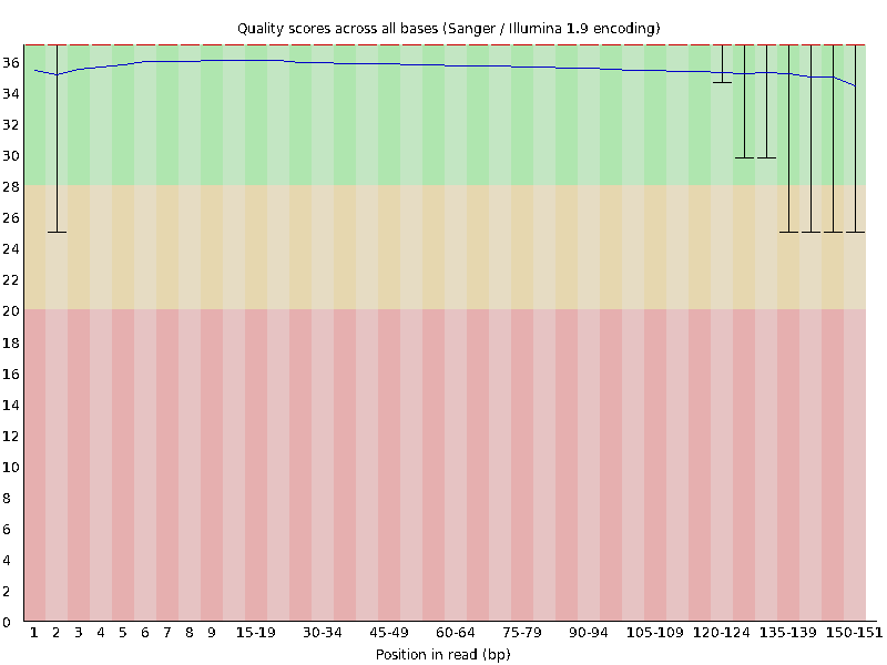
First we will look at the “Per base sequence quality” graphs for ERR4998593_1.fastq and ERR4998593_2.fastq.
| ERR4998593_1.fastq | ERR4998593_2.fastq |
|---|---|
 |
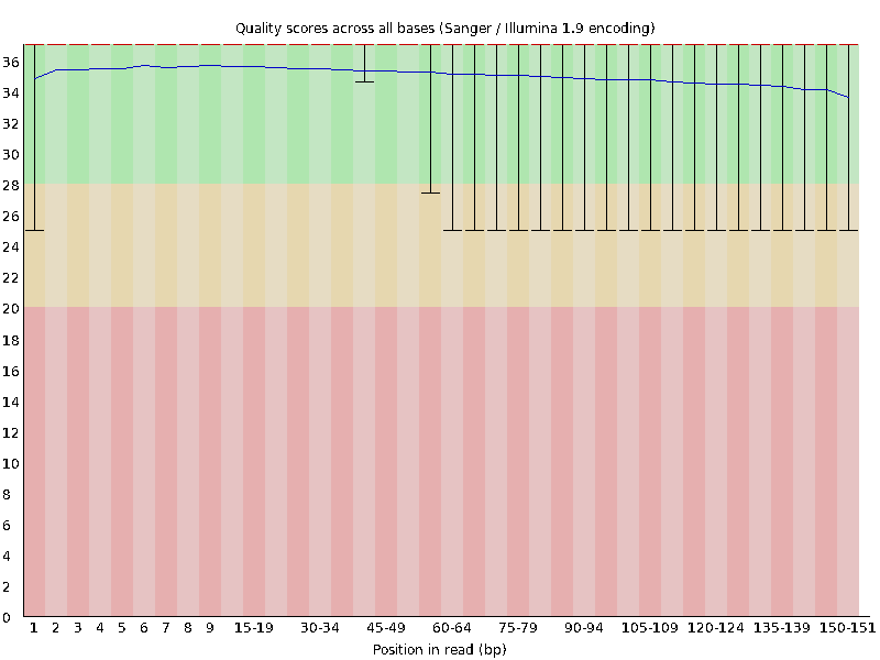 |
The x-axis displays the base position in the read, and the y-axis shows quality scores. The blue line represents the mean quality across samples.
In both samples, the mean quality values do not drop much lower than 34 at any position. This is a high quality score meaning the sequences are high quality. That means that we do not need to do any filtering. Lucky us!
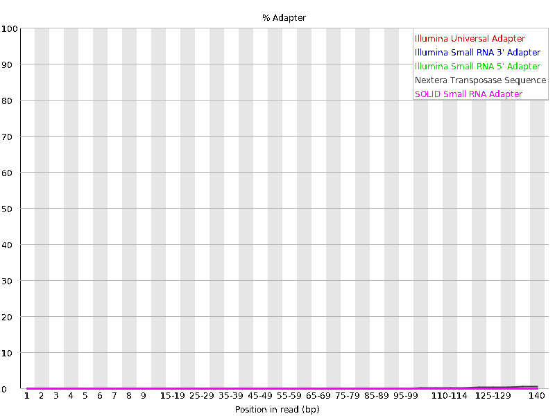
We should also have a look at the “Adapter Content” graph which will show us where adapter sequences occur in the reads. Adapter sequences are short sequences that are added to the sample to aid during the preparation of the DNA library. They therefore don’t tell us anything biologically important and should be removed if they are present in high numbers. They might also be removed in the case of certain applications, such as when the base sequence needs to be particularly accurate.
| ERR4998593_1.fastq | ERR4998593_2.fastq |
|---|---|
 |
 |
This graph shows us that these sequencing file have a low percentage (~1-2%) of adapter sequences in the reads, which means we do not need to trim any adapter sequences either.
When sequencing is poor(er) Quality
While the sequencing in this example is high quality this will not always be the case.
The programe cutadapt can be used to filter poor quality reads and trim poor quality bases. See Genomics - Trimming and Filtering to learn more about trimming and filtering poor quality reads.
Nanopore quality control
Next we will assess the quality of the Nanopore raw reads. These are found in the file located at ~/cs_course/data/nano_fastq/ERR5000342_sub12.fastq.
This file contains a subset of 12% of the Nanopore reads from our site of interest (hence sub12). The reason we aren’t using all of the reads is because there are so many that our remote computer would be overwhelmed! We will be using the sub12 data for the time being, but later in the course you will be given an assembly for analysis which was assembled using the full set of reads.
Let us again view the first complete read in one of the files from our dataset by using head to look at the first four lines.
Move to the folder containing the Nanopore data:
cd ~/cs_course/data/nano_fastq/
Use head to look at the first four line of the fastq file:
head -n 4 ERR5000342_sub12.fastq
@ERR5000342.1 1 length=407
GGTATGCTTCGTTCAGTTACGTATTGCTGTTTCGTGGCTGACCAGCAACCCGGCACCGGCGCCGAAACCGGCTCGGCGGGAATCGAGGCCCACAGCGGCACCTGCGGCGCCACCGGCAGGAACGCCACCGCGACAGCGGCCAGCGCAACGGCCACCAAAGTCGTGCCATGCGGCCCGCCGCGCACCGCTAGCAACACCGACACCGCAATCGCGAGCGCACCCCCGCCGCCACTGACGCGGCGACTGCATTCGTCAGCCGATCGCGACCGTCGCGCCTAGCCAGTTGGATAACAAACGCGAGGATCCACCAGAGTGGCGAGCACTCCGGCCAGCCCGCGCACGTTGGCCCGGTCGTGCGTGCGCAGCAAGACGATGTCGGCTGCAACGAGCAATACGTAACTTCACCA
+
*-/00*CD;>AEJ4/?FF7:73../A@@?DFBA0((+&%'&'&-)-().:B:?>=FD.3HJ@A50%$$(%'$$//24%(*06A59<:BGHM:FD@@8<G@HHG/73*#-%'%)/')'&%$$8>;>=:G;BDCD*'7B)-<<:CC6355=48BC76C=;.6B9751+,((('')89?;A@@B943BA540.+5<>>DEA87AEEA4?CDIA792*.G<B<LGDD@ALL@8:;><98:?=&*;77864C2@A>*'<;;GDCAMH;811@A@IF>A/+,'&2285>C9+(EBBC@LKDH9<;;A75H?=44-/$)12145&&('&6<=@7:@<9B6A<;A.*)213847;@B&,@C@GB?7D:B3,)18%(*-(::=?9=47A@EADHF77DHACKGA774%"%)%##$$
This read is 408 bp, longer than the Illumina reads we looked at earlier. The length of a raw read from Nanopore sequencing varies depends on the length of the length of the DNA strand being sequenced.
Line 4 shows us the quality score of this read.
*-/00*CD;>AEJ4/?FF7:73../A@@?DFBA0((+&%'&'&-)-().:B:?>=FD.3HJ@A50%$$(%'$$//24%(*06A59<:BGHM:FD@@8<G@HHG/73*#-%'%)/')'&%$$8>;>=:G;BDCD*'7B)-<<:CC6355=48BC76C=;.6B9751+,((('')89?;A@@B943BA540.+5<>>DEA87AEEA4?CDIA792*.G<B<LGDD@ALL@8:;><98:?=&*;77864C2@A>*'<;;GDCAMH;811@A@IF>A/+,'&2285>C9+(EBBC@LKDH9<;;A75H?=44-/$)12145&&('&6<=@7:@<9B6A<;A.*)213847;@B&,@C@GB?7D:B3,)18%(*-(::=?9=47A@EADHF77DHACKGA774%"%)%##$$
Based on the PHRED quality scores (see above for a reminder) we can see that the quality scores of the bases in this read range widely. Overall they are lower than the scores for Illumina reads we looked at previously.
Instead of using FastQC we will use a program called NanoPlot, which is installed on the instance, to create some plots for the whole sequencing file. NanoPlot is specially built for Nanopore sequences.
Other programs for Nanopore QC
Another popular program for QC of Nanopore reads is PycoQC.
It produces similar plots to NanoPlot but will also give you information about the overall Nanopore sequencing run. In order to generate these, PycoQC uses a
sequencing summaryfile generated by the Nanopore sequencer (e.g. MiniION or PromethION).We are using NanoPlot because the
sequencing summarythat PycoQC needs is not avaiable for this dataset. You can see example output files from PycoQC here: Guppy-2.1.3_basecall-1D_DNA_barcode.html.
We first need to navigate to the qc directory we made earlier cs_course/analysis/qc.
cd ~/cs_course/analysis/qc/
We are now going to run NanoPlot with the raw Nanopore sequencing file.
First we can look at the help documenation for NanoPlot to see what options are available.
NanoPlot --help
NanoPlot Help Documentation
usage: NanoPlot [-h] [-v] [-t THREADS] [--verbose] [--store] [--raw] [--huge]m --downsample 10000
                [-o OUTDIR] [-p PREFIX] [--tsv_stats] [--maxlength N]
                [--minlength N] [--drop_outliers] [--downsample N]
                [--loglength] [--percentqual] [--alength] [--minqual N]
                [--runtime_until N] [--readtype {1D,2D,1D2}] [--barcoded]
                [--no_supplementary] [-c COLOR] [-cm COLORMAP]
                [-f {eps,jpeg,jpg,pdf,pgf,png,ps,raw,rgba,svg,svgz,tif,tiff}]
                [--plots [{kde,hex,dot,pauvre} [{kde,hex,dot,pauvre} ...]]]
                [--listcolors] [--listcolormaps] [--no-N50] [--N50]
                [--title TITLE] [--font_scale FONT_SCALE] [--dpi DPI]
                [--hide_stats]
                (--fastq file [file ...] | --fasta file [file ...] | --fastq_rich file [file ...] | --fastq_minimal file [file ...] | --summary file [file ...] | --bam file [file ...] | --ubam file [file ...] | --cram file [file ...] | --pickle pickle | --feather file [file ...])

CREATES VARIOUS PLOTS FOR LONG READ SEQUENCING DATA.

General options:
  -h, --help            show the help and exit
  -v, --version         Print version and exit.
  -t, --threads THREADS
                        Set the allowed number of threads to be used by the script
  --verbose             Write log messages also to terminal.
  --store               Store the extracted data in a pickle file for future plotting.
  --raw                 Store the extracted data in tab separated file.
  --huge                Input data is one very large file.
  -o, --outdir OUTDIR   Specify directory in which output has to be created.
  -p, --prefix PREFIX   Specify an optional prefix to be used for the output files.
  --tsv_stats           Output the stats file as a properly formatted TSV.

Options for filtering or transforming input prior to plotting:
  --maxlength N         Hide reads longer than length specified.
  --minlength N         Hide reads shorter than length specified.
  --drop_outliers       Drop outlier reads with extreme long length.
  --downsample N        Reduce dataset to N reads by random sampling.
  --loglength           Additionally show logarithmic scaling of lengths in plots.
  --percentqual         Use qualities as theoretical percent identities.
  --alength             Use aligned read lengths rather than sequenced length (bam mode)
  --minqual N           Drop reads with an average quality lower than specified.
  --runtime_until N     Only take the N first hours of a run
  --readtype {1D,2D,1D2}
                        Which read type to extract information about from summary. Options are 1D, 2D,
                        1D2
  --barcoded            Use if you want to split the summary file by barcode
  --no_supplementary    Use if you want to remove supplementary alignments

Options for customizing the plots created:
  -c, --color COLOR     Specify a valid matplotlib color for the plots
  -cm, --colormap COLORMAP
                        Specify a valid matplotlib colormap for the heatmap
  -f, --format {eps,jpeg,jpg,pdf,pgf,png,ps,raw,rgba,svg,svgz,tif,tiff}
                        Specify the output format of the plots.
  --plots [{kde,hex,dot,pauvre} [{kde,hex,dot,pauvre} ...]]
                        Specify which bivariate plots have to be made.
  --listcolors          List the colors which are available for plotting and exit.
  --listcolormaps       List the colors which are available for plotting and exit.
  --no-N50              Hide the N50 mark in the read length histogram
  --N50                 Show the N50 mark in the read length histogram
  --title TITLE         Add a title to all plots, requires quoting if using spaces
  --font_scale FONT_SCALE
                        Scale the font of the plots by a factor
  --dpi DPI             Set the dpi for saving images
  --hide_stats          Not adding Pearson R stats in some bivariate plots

Input data sources, one of these is required.:
  --fastq file [file ...]
                        Data is in one or more default fastq file(s).
  --fasta file [file ...]
                        Data is in one or more fasta file(s).
  --fastq_rich file [file ...]
                        Data is in one or more fastq file(s) generated by albacore, MinKNOW or guppy
                        with additional information concerning channel and time.
  --fastq_minimal file [file ...]
                        Data is in one or more fastq file(s) generated by albacore, MinKNOW or guppy
                        with additional information concerning channel and time. Is extracted swiftly
                        without elaborate checks.
  --summary file [file ...]
                        Data is in one or more summary file(s) generated by albacore or guppy.
  --bam file [file ...]
                        Data is in one or more sorted bam file(s).
  --ubam file [file ...]
                        Data is in one or more unmapped bam file(s).
  --cram file [file ...]
                        Data is in one or more sorted cram file(s).
  --pickle pickle       Data is a pickle file stored earlier.
  --feather file [file ...]
                        Data is in one or more feather file(s).

EXAMPLES:
    NanoPlot --summary sequencing_summary.txt --loglength -o summary-plots-log-transformed
    NanoPlot -t 2 --fastq reads1.fastq.gz reads2.fastq.gz --maxlength 40000 --plots hex dot
    NanoPlot --color yellow --bam alignment1.bam alignment2.bam alignment3.bam --downsample 10000
We will use four flags when we run the NanoPlot command:
-
--fastqto specify the filetype and file to analyse. The raw Nanopore data is in the location/cs_course/p/data/nano_fastq/ERR5000342_sub12.fastqand we will use this full absolute path in the NanoPlot command. -
--outdirto specify the where the output files should be written. We are going to specifynano_qcso that NanoPlot will create a new directory in our current directory (qc) and write its output files to it. Note: with NanoPlot you don’t need to create this directory before running the command. -
--threadsspecifies how many threads to run the program on (more threads = more compute power = faster). We will specify 4 to indicate that four threads should be used. -
--loglengthspecifies that we want plots with a log scale.
NanoPlot --fastq ~/cs_course/data/nano_fastq/ERR5000342_sub12.fastq --outdir nano_qc --threads 4 --loglength
Now we have the command set up we can press enter and wait for NanoPlot to finish.
This will take a couple of minutes. You will know it is finished once your terminal prompt has returned (i.e. you can type in the terminal again).
Once NanoPlot has finished we can have a look at the output.
First we need to navigate into the nano_qc directory NanoPlot created, then list the files.
cd nano_qc
ls
LengthvsQualityScatterPlot_dot.html            LengthvsQualityScatterPlot_loglength_kde.png         Non_weightedLogTransformed_HistogramReadlength.png
LengthvsQualityScatterPlot_dot.png             NanoPlot_202303307_1630.log                           WeightedHistogramReadlength.html
LengthvsQualityScatterPlot_kde.html            NanoPlot-report.html                                 WeightedHistogramReadlength.png
LengthvsQualityScatterPlot_kde.png             NanoStats.txt                                        WeightedLogTransformed_HistogramReadlength.html
LengthvsQualityScatterPlot_loglength_dot.html  Non_weightedHistogramReadlength.html                 WeightedLogTransformed_HistogramReadlength.png
LengthvsQualityScatterPlot_loglength_dot.png   Non_weightedHistogramReadlength.png                  Yield_By_Length.html
LengthvsQualityScatterPlot_loglength_kde.html  Non_weightedLogTransformed_HistogramReadlength.html  Yield_By_Length.png
We can see that NanoPlot has generated a lot of different files.
Like before, we can’t view most of these files in our terminal as we can’t open images or HTML files. Instead we’ll download the core information to our own computer.
Luckily, the NanoPlot-report.html file contains all of the plots and information held in the other files so we only need to download that one onto our local computer using scp.
Use a terminal that is not logged into the cloud instance and ensure you are in your cloudspan directory. You may have one from earlier. If you do not, unveil the instructions below to start one.
Starting a new terminal
Open your file manager and navigate to the
cloudspanfolder which should contain the login key file- Open your machine’s command line interface: Windows users: Right click anywhere inside the blank space of the file manager, then select Git Bash Here. Mac users: Open Terminal and type
cdfollowed by the absolute path that leads to yourcloudspanfolder. Press enter.- Check that you are in the right folder using
pwd
Use scp to copy the file - the command will look something like:
scp -i login-key-instanceNNN.pem csuser@instanceNNN.cloud-span.aws.york.ac.uk:~/cs_course/analysis/qc/nano_qc/NanoPlot-report.html .
Remember to replace NNN with the instance number specific to you. As the file is downloading you will see an output like:
scp -i login-key-instanceNNN.pem csuser@instanceNNN.cloud-span.aws.york.ac.uk:~/cs_course/analysis/qc/nano_qc/NanoPlot-report.html .
NanoPlot-report.html                                  100% 3281KB   2.3MB/s   00:01
Once the file has downloaded, use the File Explorer (Windows) or Finder (Mac) to find the file and open it - it should open up in your browser.
Help!
If you had trouble downloading and viewing the file you can view it here: NanoPlot-report.html
In the report we can view summary statistics followed by plots showing the distribution of read lengths and the read length vs average read quality.
Looking at the summary statistics table answer the following questions:
Exercise 1:
- How many sequences are in this file?
- How many bases are there in this entire file?
- What is the length of the longest read in the file and its associated mean quality score?
Solution
- There are 316,251 sequences (also known as reads) in this file
- There are 1,324,863,094 bases (bp) in total in this FASTQ file
- The longest read in this file is 49893 bp and it has a mean quality score of 9.3
Quality Encodings Vary
Note that not all sequencing machines use the same encoding for quality. So
#might not always mean 3, a poor quality score.This means it’s essential that you know which sequencing platform was used to generate your data, so that you can tell your quality control program which encoding to use. If you choose the wrong encoding, you run the risk of throwing away good reads or (even worse) not throwing away bad reads! Nanopore quality encodings are no exception. You can read more about the differences with Nanopore sequencing here: EPI2ME - Quality Scores.
N50
The N50 length is a useful statistic when looking at sequences of varying length as it indicates that 50% of the total sequence is in reads (i.e. chunks) that are that size or larger.
For this FASTQ file 50% of the total bases are in reads that have a length of 5,974 bp or longer.
See the webpage What’s N50? for a good explanation. We will be coming back to this statistic in more detail when we get to the assembly step.
We can also look at some of the plots produced by NanoPlot.
One useful plot is the plot titled “Read lengths vs Average read quality plot using dots after log transformation of read lengths”.
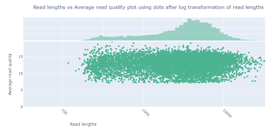
This plot shows the average quality of the sequence against the read lengths. We can see that the majority of the sequences have a quality score at least 7. We don’t necessarily need to trim these reads, as this is a good score, but we will do it anyway to show you how.
Filtering Nanopore sequences by quality score
We can use the program Seqkit (which contains many tools for FASTQ/A file manipulation) to filter our reads. We will be using the command seqkit seq to create a new file containing only the sequences with an average quality above a certain value.
After returning to our nano_fastq directory, we can view the seqkit seq help documentation with the following command:
cd ~/cs_course/data/nano_fastq
seqkit seq -h
Seqkit seq help documentation
transform sequences (extract ID, filter by length, remove gaps...)

Usage:
  seqkit seq [flags]

Flags:
  -k, --color                     colorize sequences - to be piped into "less -R"
  -p, --complement                complement sequence, flag '-v' is recommended to switch on
      --dna2rna                   DNA to RNA
  -G, --gap-letters string        gap letters (default "- \t.")
  -h, --help                      help for seq
  -l, --lower-case                print sequences in lower case
  -M, --max-len int               only print sequences shorter than the maximum length (-1 for no limit) (default -1)
  -R, --max-qual float            only print sequences with average quality less than this limit (-1 for no limit) (default -1)
  -m, --min-len int               only print sequences longer than the minimum length (-1 for no limit) (default -1)
  -Q, --min-qual float            only print sequences with average quality qreater or equal than this limit (-1 for no limit) (default -1)
  -n, --name                      only print names
  -i, --only-id                   print ID instead of full head
  -q, --qual                      only print qualities
  -b, --qual-ascii-base int       ASCII BASE, 33 for Phred+33 (default 33)
  -g, --remove-gaps               remove gaps
  -r, --reverse                   reverse sequence
      --rna2dna                   RNA to DNA
  -s, --seq                       only print sequences
  -u, --upper-case                print sequences in upper case
  -v, --validate-seq              validate bases according to the alphabet
  -V, --validate-seq-length int   length of sequence to validate (0 for whole seq) (default 10000)

Global Flags:
      --alphabet-guess-seq-length int   length of sequence prefix of the first FASTA record based on which seqkit guesses the sequence type (0 for whole seq) (default 10000)
      --id-ncbi                         FASTA head is NCBI-style, e.g. >gi|110645304|ref|NC_002516.2| Pseud...
      --id-regexp string                regular expression for parsing ID (default "^(\\S+)\\s?")
      --infile-list string              file of input files list (one file per line), if given, they are appended to files from cli arguments
  -w, --line-width int                  line width when outputting FASTA format (0 for no wrap) (default 60)
  -o, --out-file string                 out file ("-" for stdout, suffix .gz for gzipped out) (default "-")
      --quiet                           be quiet and do not show extra information
  -t, --seq-type string                 sequence type (dna|rna|protein|unlimit|auto) (for auto, it automatically detect by the first sequence) (default "auto")
  -j, --threads int                     number of CPUs. can also set with environment variable SEQKIT_THREADS) (default 4)
From this we can see that the flag -Q will “only print sequences with average quality qreater or equal than this limit (-1 for no limit) (default -1)”.
From the plot above we identified that most of the reads had a quality score of at least 7. To make sure some filtering happens, we’ll use a minimum limit of 8.
seqkit seq -Q 8 ERR5000342_sub12.fastq > ERR5000342_sub12_filtered.fastq
In the command above we use redirection (>) to generate a new file data/nano_fastq/ERR5000342_sub12_filtered.fastq containing only the reads with an average quality of 8 or above.
We can now re-run NanoPlot on the filtered file to see how it has changed.
cd ~/cs_course/analysis/qc/

NanoPlot --fastq ~/cs_course/data/nano_fastq/ERR5000342_sub12_filtered.fastq --outdir nano_qc_filt --threads 4 --loglength
Once again, wait for the command to finish and then scp the report to your local computer. First, though, make sure you rename the file so you know which is the filtered report and which isn’t.
cd nano_qc_filt
mv NanoPlot-report.html NanoPlot-report-filtered.html
Help!
If you had trouble downloading the file you can view it here: NanoPlot-filtered-report.html
Compare the NanoPlot statistics of the Nanopore raw reads before filtering and after filtering and answer the questions below.
Exercise 2:
- How many reads have been removed by filtering?
- How many bases have been removed by filtering?
- What is the length of the new longest read and its associated average quality score?
Solution
- Initially there were 316,251 reads; in the filtered file there are 311,172 reads; so 5079 reads have been removed by the quality filtering
- Initially there were 1,324,863,094 bases and after filtering there are 1,303,931,978 base which means filtering has removed 20,931,116 bases
- The longest read in the filtered file is the same as before: 49893bp and it has a mean quality score of 9.3.
Key Points
Quality encodings vary across sequencing platforms.
It is important to know the quality of our data to be able to make decisions in the subsequent steps.
Data cleaning is essential at the beginning of metagenomics workflows.
Due to differences in the sequencing technology Nanopore data must be handled differently.