Introduction to Metagenomics
Overview
Teaching: 30 min
Exercises: 5 minQuestions
What is metagenomics?
When should we use metagenomics?
What does a metagenomics project look like?
Objectives
Explain the difference between genomics, metagenomics and amplicon sequencing.
Familiarise yourself with the metagenomics dataset used in this course.
What is the difference between Genomics and Metagenomics?
In genomics, we sequence and analyse the genome of a single species. We often have a known reference genome to which we can align all our reads.
In metagenomics we sequence samples composed of many genomes. These might be environmental samples from soil or anaerobic digestors for example, or samples from the skin or digestive tracts of animals. Such samples typically include species that are difficult to culture and thus lack reference genomes. The challenge in metagenomics is to assemble this mix of diverse genomes into its constituent genomes.
Metagenomics
A metagenome is a collection of genomic sequences from various (micro) organisms coexisting in a given space. They are snapshots that tell us about the taxonomic, metabolic or functional composition of the communities that we study.
Analysing multiple genomes rather than individual genomes introduces additional complexity:
- Taxonomic assignment: How can we separate the sequences to the different putative organisms or taxonomic units?
- Community Composition: How can we quantify the relative abundances of the taxonomic units present?
A typical metagenomic workflow is designed to answer two questions:
- What species are present in the sample and what are their relative abundances?
- What is the functional capacity of the organisms or the community?
Community sequencing approaches
There are two technologies used in mixed community sequencing which have different use cases, advantages and disadvantages: Whole genome metagenomics and Amplicon/(16S) sequencing.
Whole metagenome sequencing (WMS)
Random parts of all of the genomes present in a sample are sequenced in WMS. We aim to find what organism, or “taxonomic unit”, they come from, what part of their genome they come from, and what functions they encode. This can be done by cross-referencing the sequences obtained with databases of information.
If the metagenome is complex and deeply sequenced enough, we may even be able obtain full individual genomes from WMS and a strong understanding of the functional capacity of the microbiome.
For abundant organisms in a metagenome sample, there are likely to be enough data to generate reasonable genome coverage. However, this is not the case for low abundance organisms. Often deeper sequencing/ more total sequencing data is required to assemble the genomes of these organisms. If your research question can be addressed by considering the most abundant organisms, you need do less sequencing than if your question requires an understanding of the rarest organisms present.
The cost of both preparing the samples and the computational effort required to analyse them can become prohibitively expensive quickly. Before starting you need to think carefully about the question your dataset is trying to answer and how many samples you will need to sequence to get one. This is especially the case when you are trying to include biological or technical replication in your experimental design.
Amplicon sequencing
An amplicon is a small piece of DNA or RNA that will be amplified through PCR (Polymerase Chain Reaction). Amplicon sequencing is cheaper than WMS because only a small part of the genome is sequenced. This makes it affordable to include additional replicates.
The region being amplified needs to be present in all the individuals in the community being characterised, and be highly conserved. 16 rRNA is often used for amplicon sequencing in bacteria for this reason (for eukaryotes 18S rRNA is used instead).
For organisms that are well characterised, establishing identity can give you information about functional capacity of the community. For organisms which are not well characterised - and these are common in such samples - we will know little other than relative abundances in the community.
Despite this, there are workflows such as QIIME2, which are free and community led, which use database annotations of the reference versions of the organisms identified from the amplicon, to suggest what metabolic functions maybe present. The amplicon sequence is also limited because species may have genomic differences, but may be indistinguishable from the amplicon sequence alone. This means that amplicon sequencing can rarely resolve to less than a genus level.
| Attribute | Amplicon | Whole genome metagenomics |
|---|---|---|
| Cost | Cheap | Expensive |
| Coverage depth | High | Lower - medium |
| Taxonomy detection | Specific to amplicons used | All in sample |
| Genome coverage | Only region amplified | All of genome |
| Taxonomic resolution | Lower | Higher |
| Turnaround time | Fast | Slower - more computational time for analysis needed |
Nanopore (long-read) vs Illumina (short-read) data
In our Statistically Useful Experimental Design course we cover how to choose your sequencing platform based on your research question. However, it’s a bit different when doing a whole metagenome assembly experiment.
For single genome analyses you can choose between assembling your genome one of two ways: using a reference as a template or de novo (without a reference). Which route you choose depends on whether there is a reasonable reference available for the genome you’re assembling.
When looking at whole metagenome assembly, there will not be a reference available for the metagenome as a whole. You are also unlikely to know what species will be present. All of your assembly stages will therefore be de novo. This makes using long reads preferable as it’s easier to piece them together.
We will talk about this more later in this lesson as part of the Genome Assembly section. There are pros and cons to each using both long and short reads, and so using them in combination is usually the best method. These pros and cons are irrespective of the application.
However, for metagenome analysis, if you were to use only short read sequencing for the assembly you would end up with a much more fragmented assembly to work with.
| Short reads | Long reads | |
|---|---|---|
| Technologies | Illumina | Nanopore and pacbio |
| Number of reads generated | 800 million paired end* | Depends on read length, and instrument, but usually only 10s of thousands** |
| Base accuracy | Very high | Low |
| Ease of assembly | Very difficult | Easier |
| Format output files | Fastq | Fastq, Fast5 |
| Read length | 150-300bp | Commonly 10-30kb*** |
* As of July 2022, the NextSeq 550 high-output system runs were capable of generating upto 800 million paired-end reads in one run
** There are different Nanopore instruments. The smaller instruments, like the minION, will generate far fewer reads. Larger instruments like the promethION will result in ~10-20k reads, but this will vary a lot between samples and their quality. They will never result in millions of reads like the Illumina platforms.
*** The read length will vary based on the DNA extraction method. If the DNA is very fragmented it will not result in very long reads. In many metagenomes bead beating is required to lyse cells, and so read length will still be longer than Illumina but shorter than non-metagenomic samples sequenced.
Our data
The data we will be using for the rest of the course (and that we’ve been using already!) comes from a 2022 paper titled In-depth characterization of denitrifier communities across different soil ecosystems in the tundra.
The paper looks at microbial communities across 43 mountain tundra sites in Northern Finland. The researchers took soil samples from each site and followed a metagenomic analysis workflow to identify the species present in each one. They also measured environmental information such as elevation, soil moisture and N2O fluxes.
We will be focusing on data from a single heathland site which has two sets of sequencing data available: one long-read (nanopore) and one short-read (illumina). We’ve already taken a look at these data as part of the previous two lessons - they are saved on our cloud instance under nano_fastq and illumina_fastq respectively.
Towards the end of the course we’ll compare some of the data from our site with another site to see how they differ in terms of species composition and diversity.
Bioinformatic workflows
When working with high-throughput sequencing data, the raw reads you get off of the sequencer need to pass through a number of different tools in order to generate your final desired output.
The use of this set of tools in a specified order is commonly referred to as a workflow or a pipeline.
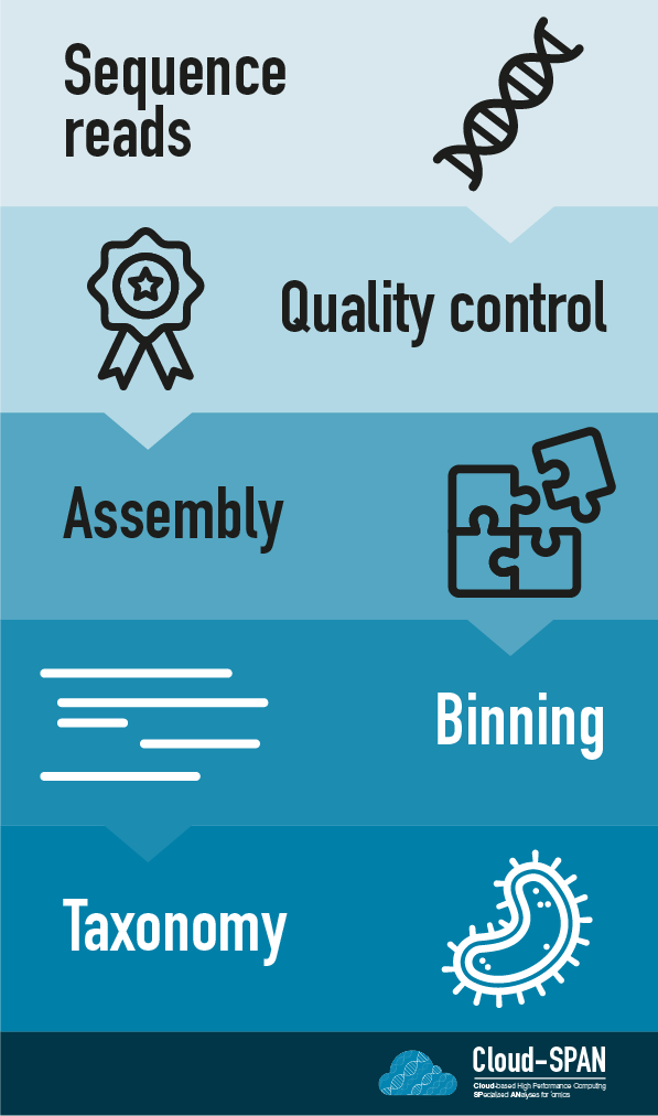
Here is an example of the workflow we will be using for our analysis with a brief description of each step.
- Sequence reads - obtaining raw reads from a sample via sequencing
- Quality control - assessing quality of the reads and trimming and filtering if necessary.
- Metagenome assembly - piecing together genomes from reads into multiple long “contigs” (overlapping DNA segments)
- Binning - separating out genomes into ‘bins’ containing related contigs
- Taxonomic assignment - assigning taxonomy and functional analysis to sequences/contigs
Workflows in bioinformatics often adopt a plug-and-play approach so the output of one tool can be easily used as input to another tool. The use of standard data formats in bioinformatics (such as FASTA or FASTQ, which we will be using here) makes this possible. The tools that are used to analyze data at different stages of the workflow are therefore built under the assumption that the data will be provided in a specific format.
You can find a more detailed version of the workflow we will be following by going to Extras and selecting Workflow Reference. This diagram contains all of the steps followed over the course alongside program names.
Next steps
Hopefully you now feel ready to start following our workflow to analyse our data. We’ll be guiding you through the steps and giving more context for each one as we go along. Let’s go!
Key Points
Genomics looks at the whole genome content of an organism
Metagenomes contain multiple organisms within one sample unlike genomic samples.
In metagenomes the organisms present are not usually present in the same abundance - except for mock communities.
We can identify the organisms present in a sample using either amplicon sequencing or whole metagenome sequencing. Amplicon sequencing is cheaper and quicker, but it also limits the amount of downstream analysis that can be done with the data.
Metagenomes can differ in their levels of complexity and this is determined by how many organisms are in the metagenome.
Difference platforms allow us to perform different analyses. The suitability depends on the question you are asking.