Introduction to Metagenomics
Overview
Teaching: 30 min
Exercises: 5 minQuestions
What is metagenomics?
When should we use metagenomics?
What does a metagenomics project look like?
Objectives
Explain the difference between genomics, metagenomics and amplicon sequencing.
Familiarise yourself with the metagenomics dataset used in this course.
What is the difference between Genomics and Metagenomics?
In genomics, we sequence and analyse the genome of a a single species. We often have a known reference genome to which we can align all our reads. In metagenomics we sequence samples composed of many genomes. These might be environmental samples from soil or anaerobic digestors for example, or samples from the skin or digestive tracts of animals. Such samples typically include species that are difficult to culture and thus lack reference genomes. The challenge in metagenomics is to assemble this mix of genomes into separate genomes.
Metagenomics
A metagenome is a collection of genomic sequences from various (micro) organisms coexisting in a given space. They are snapshots that tell us about the taxonomic, metabolic or functional composition of the communities that we study.
Analysing multiple genomes rather than individual genomes introduces additional complexity:
- Taxonomic assignment: How can we separate the sequences to the different putative organisms or taxonomic units
- Community Composition: How can we quantify the relative abundances of the taxonomic units present
A typical metagenomic workflow is designed to answer two questions:
- What species are present in the sample and what are their relative abundances?
- What is the functional capacity of the organisms or the community?
Community sequencing approaches
There are two technologies used in mixed community sequencing which have different use cases, advantages and disadvantages: Whole genome metagenomics and Amplicon/(16S) sequencing.
Whole metagenome sequencing (WMS)
Random parts of the all of genomes present in a sample are sequenced in WGS. We aim to find what organism, or taxonomic unit, they come from, what part of their genome they come from, and what functions they encode.
Depending on the complexity of the metagenome and the amount of sequencing done, we may be able obtain full individual genomes from WMS and a strong understanding of the functional capacity of the microbiome.
For abundant organisms in a metagenome sample, there are likely to be enough data to generate reasonable genome coverage. However, this is not the case for low abundance organisms. Often deeper sequencing/ more total sequencing data is required to assemble the genomes of these organisms. If you research question can be addressed by considering the most abundant organisms, you need do less sequencing than if you question requires an understanding of the rarest organisms.
Depending on the question your dataset is trying to answer and how many samples you will need to sequence, the cost of both preparing the samples and the computational effort required to analyse them can become prohibitively expensive quickly. This is especially the case when you are trying to include biological or technical replication in your experimental design.
Amplicon sequencing
An amplicon is a small piece of DNA or RNA that will be amplified. Amplicon sequencing is cheaper than WMS because only a smal part of the genome is sequenced. This makes it affordable to include additional replicates. Because only one small region is amplified through PCR, rather than the whole genome, the region needs to be present in all the individuals in the community that you want to identify. Consequently, we use 16S rRNA which is part of every bacterial and archaeal genome and is highly conserved, to identify bacteria and archeae. 18S rRNA or ITS regions are the amplicons used to identify eukarotic organisms.
For organisms that are well characterised, establishing identity can give you information about functional capacity of the community. For organisms which are not well characterised - and these are common in such samples - we will know little other than relative abundances in the community.
Despite this, there are workflows such as QIIME2, which are free and community led, which use database annotations of the reference versions of the organisms identified from the amplicon, to suggest what metabolic functions maybe present. The amplicon sequence is also limited because species may have genomic differences, but may be indistinguishable from the amplicon sequence alone. This means that amplicon sequencing can rarely resolve to less than a genus level.
| Attribute | Amplicon | Whole genome metagenomics |
|---|---|---|
| Cost | Cheap | Expensive |
| Coverage depth | High | Lower - medium |
| Taxonomy detection | Specific to amplicons used | All in sample |
| Genome coverage | Only region amplified | All of genome |
| Taxonomic resolution | lower | higher |
| Turnaround time | Fast | Slower - more computational time for analysis needed |
Bioinformatic workflows
When working with high-throughput sequencing data, the raw reads you get off of the sequencer need to pass through a number of different tools in order to generate your final desired output.
The use of this set of tools in a specified order is commonly referred to as a workflow or a pipeline.
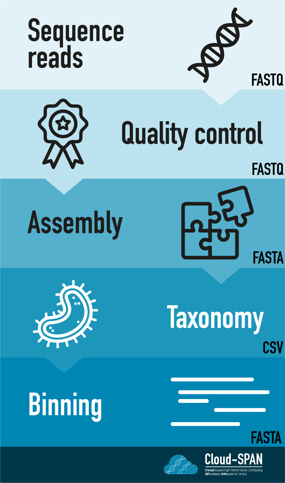
Here is an example of the workflow we will be using for our analysis with a brief description of each step.
- Sequence reads - obtaining raw reads from a sample via sequencing
- Quality control - assessing quality using FastQC, and trimming and/or filtering reads (if necessary)
- Metagenome assembly - piecing together genomes from reads using Flye, a long-read metagenome assembler
- Binning - separating out genomes into ‘bins’ containing related contigs using Metabat2
- Taxonomic assignment - assigning taxonomy to sequences/contigs using Krona and/or Pavion
Workflows in bioinformatics often adopt a plug-and-play approach so the output of one tool can be easily used as input to another tool. The use of standard data formats in bioinformatics (such as FASTA or FASTQ, which we will be using here) makes this possible. The tools that are used to analyze data at different stages of the workflow are therefore built under the assumption that the data will be provided in a specific format.
You can find a more detailed version of the workflow we will be following by going to Extras and selecting Workflow Reference. This diagram contains all of the steps followed over the course alongside program names.
Metagenome complexity
As the number of organisms increases in a community so does the complexity. See Pimm , 1984 for an explanation of community complexity.
A low-complexity microbial community is made up of fewer organisms and as a result the metagenomic data is usually easier to process and analyse than a high-complexity microbial community.
There’s no official definition for what makes a community low or high complexity. But some examples of a low complexity microbial community include natural whey starter cultures, made up of around three different organisms, which are used in cheese production: see Somerville et al., 2019.
Defining our community
How many organisms are in the mock metagenome community we are using? Do you think this is high or low complexity compared to your own samples?
Solution
There are 10 species. This is low complexity compared to the human gut microbiome which itself is low compared to a soil microbiome.
Mock metagenomes versus real samples
People often use publically available sequencing data to perform analyses or for testing an analysis pipeline on a smaller or similar dataset.
However mock metagenomes are communities that are made by combining known species at known quantities to generate a mock sample. This mock community is often much simpler than a real metagenome, however it can be useful to know exactly what is in a metagenome, in order to test whether the result we get is sensible.
One reason for using these mock samples would be to test a workflow. The simplicity and quality of mock metagenome data means that performing analysis on these mock samples can be much easier computationally, and run more quickly.
However the main reason for using mock samples are to benchmark developing software tools. If you are aware of the level of complexity in a sample, and you know the content of the community, it is easier for you to identify false positives and false negatives.
Some mock datasets, like the one we will be using for this course, have the organisms present with log fold differences in the abundance between the organisms. This is much more representative of a real community compared to a mock community, where all organisms are present at the same abundance. However it is useful to know that this is still an “idealised” dataset. In most cases the samples will not contain all known organisms, and often there will be degraded pieces of DNA in there.
Dataset used in this course
This course uses data from a mock metagenome community published from Ultra-deep, long-read nanopore sequencing of mock microbial community standards which has long and short read sequencing data and has been used for benchmarking metagenome tools.
This community contains eight bacteria (three gram positive and five gram negative) and two yeasts. These organisms are present in log abundances relative to each other. The organisms present and their known percentage of the total metagenome content is given in the table below.
This dataset contains whole metagenome sequencing. The short read data are generated on the Illumina platform and the long reads are generated using Oxford Nanopore Technology’s Nanopore platform. Other popular long read sequencing platforms exist, such as PacBio, though we will not be covering PacBio specific methodology here. Despite this, the same principle stages exist in the workflow, and often only different parameters are required to adapt analysis to different platforms.
| Species | Genomic DNA % | Genome coverage |
|---|---|---|
| Listeria monocytogenes | 89.1 | 94.8 |
| Pseudomonas aeruginosa | 8.9 | 4.2 |
| Bacillus subtilis | 0.89 | 0.7 |
| Saccharomyces cerevisiae | 0.89 | 0.23 |
| Escherichia coli | 0.089 | 0.058 |
| Salmonella enterica | 0.089 | 0.059 |
| Lactobacillus fermentum | 0.0089 | 0.015 |
| Enterococcus faecalis | 0.00089 | 0.001 |
| Cryptococcus neoformans | 0.00089 | 0.00015 |
| Staphylococcus aureus | 0.000089 | 0.0001 |
Differences between nanopore and illumina data
Elsewhere (see here)we have covered information about how to use your research question to guide your preference of platform (Illumina/Nanopore)when designing an experiment. However typically the equivalent question for metagenomics is whether to sequence the whole genome, or whether amplicon sequencing will be preferable.
For non-metagenomic analyses, you can choose to do either a reference based or de novo approach for assembly. This will be dependent on whether there is a reasonable reference for your organism.
However, for whole metagenome sequencing, reference genomes will exist that can be compared to organisms identified from your metagenome. However, this will be at the binning stage and a reference will not exist for your metagenome as a whole. Due to this, all of the assembly stages of the metagenome analysis pipeline are de novo. As a result, there is a bigger advantage to using long read sequencing over short read sequencing to assemble a metagenome if you were to choose only one method.
This will be covered in the Genome Assembly section of this course. There are pros and cons to each using both long and short reads, and so using them in combination is usually the best method. These pros and cons are irrespective of the application.
However, for metagenome analysis, if you were to use only short read sequencing for the assembly you would end up with a much more fragmented assembly to work with.
| Short reads | Long reads | |
|---|---|---|
| Technologies | Illumina | Nanopore and pacbio |
| Number of reads generated | 800 million paired end* | Depends on read length, and instrument, but usually only 10s of thousands** |
| Base accuracy | Very high | Low |
| Ease of assembly | Very difficult | Easier |
| Format output files | Fastq | Fastq, Fast5 |
| Read length | 150-300bp | Commonly 10-30kb*** |
* As of July 2022, the NextSeq 550 high-output system runs were capable of generating upto 800 million paired-end reads in one run
** There are different Nanopore instruments. The smaller instruments, like the minION, will generate far fewer reads. Larger instruments like the promethION will result in ~10-20k reads, but this will vary a lot between samples and their quality. They will never result in millions of reads like the Illumina platforms.
*** The read length will vary based on the DNA extraction method. If the DNA is very fragmented it will not result in very long reads. In many metagenomes bead beating is required to lyse cells, and so read length will still be longer than Illumina but shorter than non-metagenomic samples sequenced.
Key Points
Genomics looks at the whole genome content of an organism
Metagenomes contain multiple organisms within one sample unlike genomic samples.
In metagenomes the organisms present are not usually present in the same abundance - except for mock communities.
We can identify the organisms present in a sample using either amplicon sequencing or whole metagenome sequencing. Amplicon sequencing is cheaper and quicker, however it also limits the amount of downstream analysis that can be done with the data.
Metagenomes can differ in their levels of complexity and this is determined by how many organisms are in the metagenome.
Difference platforms allow us to perform different analyses. The suitability depends on the question you are asking.