Functional annotation
Overview
Teaching: 40 min
Exercises: 10 minQuestions
How can we add functional annotation to our bins?
Objectives
Define what funtional annotation is
Know how to use prokka for functional annotation
What is functional annotation?
Now we have our binned MAGs, we can start to think about what functions genes contained within their genomes do. We can do this via functional annotation - a way to collect information about and describe a DNA sequence.
Next lesson we will talk about taxonomic annotation, which tells us which organisms are present in the metagenome assembly. This lesson, however, we will do some brief functional annotation to get more information about the potential metabolic capacity of the organism we are annotating. This is possible because there is software available which uses features in DNA sequences to predict where genes start and end, allowing us to predict which genes are in our MAGs.
A high quality functional annotation is important because it is very useful for lots of downstream analyses. For instance, if we were looking for genes that have a particular function, we would only be able to do that if we were able to predict the location of the genes in these assemblies.
For example, the paper this data is pulled from uses functional annotation of MAGs to look for genes associated with denitrification pathways. The abundance of these genes is then linked to N2O flux rates at different sites.
In this lesson we will only be doing a very small amount of functional annotation using the tool Prokka for rapid prokaryotic genome annotation. This is intended as a taster to give you an idea what you can use your MAGs for. There are many other routes to be taken regarding functional annotation, some of which will be discussed briefly at the end of this episode.
As with taxonomic annotation, effectiveness is determined by the database that the MAG sequence is being compared to. If you do not use the appropriate database you may not end up with many annotated sequences. In particular, Prokka (the tool we will use in this episode) annotates archaea and bacterial genomes. If you are trying to annotate a fungal genome or a eukaryote, you will need to use something different.
How do we perform functional annotation?
Software choices
We are using Prokka here as it is still the software most commonly used. However, the program is no longer being updated. One recent alternative that is being actively developed is Bakta.
Prokka identifies candidate genes in a iterative process. First it uses Prodigal (another command line tool) to find candidate genes.These are then compared against databases of known protein sequences in order to determine their function. If you like, you can read more about Prokka in this 2014 paper.
Prokka has been pre-installed on our instance. First, let’s create a directory inside analysis where we can store our outputs from Prokka.
cd ~/cs_course/analysis/
mkdir prokka
cd prokka
For now we will annotate just one MAG at a time with Prokka. In the previous episode we produced 90 MAGs of varying quality. In this example, we will start with the MAG bin.45.fa, as this MAG had the fairly high completeness (57.76%) and only 1.72% contamination.
Before we start we’ll need to activate a conda environment to run the software.
Activating an environment
Environments are a way of installing a piece of software so that it is isolated, so that things installed within an environment, do not affect other software installed at system wide level. For some pieces of software, the requirements for different dependency versions, such different versions of python mean this is an easy way to have multiple pieces of software installed without conflicts. One popular way to manage environments is to use conda which is a popular environment manager. We will not discuss using conda in detail, so for further information of how to use it, here is a Carpentries course that covers how to use conda in more detail.
For this course we have created a conda environment containing prokka. In order to use this we will need to use the conda activate command:
conda activate prokka
You will be able to tell you have activated your environment because your prompt should go from looking like this, with (base) at the beginning…
(base) csuser@instance001:~ $
…to having (prokka) at the beginning. If you forget whether you are in an the prokka environment, look back to see what the prompt looks like.
(prokka) csuser@instance001:~ $
Now let’s take a look at the help page for Prokka using the -h flag.
prokka -h
Prokka Help documentation
Name:
 Prokka 1.12 by Torsten Seemann <torsten.seemann@gmail.com>
Synopsis:
 rapid bacterial genome annotation
Usage:
 prokka [options] <contigs.fasta>General:
 --help            This help
 --version         Print version and exit
 --docs            Show full manual/documentation
 --citation        Print citation for referencing Prokka
 --quiet           No screen output (default OFF)
 --debug           Debug mode: keep all temporary files (default OFF)
Setup:
 --listdb          List all configured databases
 --setupdb         Index all installed databases
 --cleandb         Remove all database indices
 --depends         List all software dependencies
Outputs:
--outdir [X]      Output folder [auto] (default '')
--force           Force overwriting existing output folder (default OFF)
--prefix [X]      Filename output prefix [auto] (default '')
--addgenes        Add 'gene' features for each 'CDS' feature (default OFF)
--addmrna         Add 'mRNA' features for each 'CDS' feature (default OFF)
--locustag [X]    Locus tag prefix [auto] (default '')
--increment [N]   Locus tag counter increment (default '1')
--gffver [N]      GFF version (default '3')
--compliant       Force Genbank/ENA/DDJB compliance: --addgenes --mincontiglen 200 --centre XXX (default OFF)
--centre [X]      Sequencing centre ID. (default '')
--accver [N]      Version to put in Genbank file (default '1')
Organism details:
 --genus [X]       Genus name (default 'Genus')
 --species [X]     Species name (default 'species')
 --strain [X]      Strain name (default 'strain')
 --plasmid [X]     Plasmid name or identifier (default '')
Annotations:
 --kingdom [X]     Annotation mode: Archaea|Bacteria|Mitochondria|Viruses (default 'Bacteria')
 --gcode [N]       Genetic code / Translation table (set if --kingdom is set) (default '0')
 --gram [X]        Gram: -/neg +/pos (default '')
 --usegenus        Use genus-specific BLAST databases (needs --genus) (default OFF)
 --proteins [X]    FASTA or GBK file to use as 1st priority (default '')
 --hmms [X]        Trusted HMM to first annotate from (default '')
 --metagenome      Improve gene predictions for highly fragmented genomes (default OFF)
 --rawproduct      Do not clean up /product annotation (default OFF)
 --cdsrnaolap      Allow [tr]RNA to overlap CDS (default OFF)
Computation:
 --cpus [N]        Number of CPUs to use [0=all] (default '8')
 --fast            Fast mode - only use basic BLASTP databases (default OFF)
 --noanno          For CDS just set /product="unannotated protein" (default OFF)
 --mincontiglen [N] Minimum contig size [NCBI needs 200] (default '1')
 --evalue [n.n]    Similarity e-value cut-off (default '1e-06')
 --rfam            Enable searching for ncRNAs with Infernal+Rfam (SLOW!) (default '0')
 --norrna          Don't run rRNA search (default OFF)
 --notrna          Don't run tRNA search (default OFF)
 --rnammer         Prefer RNAmmer over Barrnap for rRNA prediction (default OFF)
Looking at the help page tells us how to construct our basic command, which looks like this:
prokka --outdir mydir --prefix mygenome contigs.fa
--outdir mydirtells Prokka that the ‘output directory’ ismydir--prefix mygenometells Prokka that the output files should all be labelledmygenomecontigs.fais the file we want Prokka to annotate
Prokka produces multiple different file types, which you can see in the table below. We are mainly interested in .faa and .tsv but many of the other files are useful for submission to different databases.
| Suffix | Description of file contents |
|---|---|
| .fna | FASTA file of original input contigs (nucleotide) |
| .faa | FASTA file of translated coding genes (protein) |
| .ffn | FASTA file of all genomic features (nucleotide) |
| .fsa | Contig sequences for submission (nucleotide) |
| .tbl | Feature table for submission |
| .sqn | Sequin editable file for submission |
| .gbk | Genbank file containing sequences and annotations |
| .gff | GFF v3 file containing sequences and annotations |
| .log | Log file of Prokka processing output |
| .txt | Annotation summary statistics |
| .tsv | Tab-separated file of all features: locus_tag,ftype,len_bp,gene,EC_number,COG,product |
prokka --outdir bin.45 --prefix bin.45 ../binning/assembly_ERR5000342.fasta.metabat-bins1500-YYYMMDD_HHMMSS/bin.45.fa
This should take around 1-2 minutes on the instance so we will not be running the command in the background.
Exercise 1: Recap of Prokka command
Test yourself! What do each of these parts of the command signal?
--outdir bin.45--prefix bin.45../binning/assembly_ERR5000342.fasta.metabat-bins1500-YYYMMDD_HHMMSS/bin.45.faSolution
bin.45is the name of the directory where Prokka will place its output filesbin.45will be the name of each output file e.g.bin.45.tsvorbin.45.faa- This is the file path for the file we want Prokka to annotate
When you initially run the command you should see similar to the following.
[11:58:55] This is prokka 1.12
[11:58:55] Written by Torsten Seemann <torsten.seemann@gmail.com>
[11:58:55] Homepage is https://github.com/tseemann/prokka
[11:58:55] Local time is Wed Mar 22 11:58:55 2023
[11:58:55] You are csuser
[11:58:55] Operating system is linux
[11:58:55] You have BioPerl 1.006924
[11:58:55] System has 8 cores.
[11:58:55] Will use maximum of 8 cores.
[11:58:55] Annotating as >>> Bacteria <<<
[11:58:55] Generating locus_tag from '../binning/assembly_ERR5000342.fasta.metabat-bins1500-YYYMMDD_HHMMSS/bin.45.fa' contents.
And you should see the following when the command has finished:
[12:00:28] Output files:
[12:00:28] bin.45/bin.45.fna
[12:00:28] bin.45/bin.45.faa
[12:00:28] bin.45/bin.45.ffn
[12:00:28] bin.45/bin.45.fsa
[12:00:28] bin.45/bin.45.err
[12:00:28] bin.45/bin.45.sqn
[12:00:28] bin.45/bin.45.txt
[12:00:28] bin.45/bin.45.gbk
[12:00:28] bin.45/bin.45.tsv
[12:00:28] bin.45/bin.45.gff
[12:00:28] bin.45/bin.45.log
[12:00:28] bin.45/bin.45.tbl
[12:00:28] Annotation finished successfully.
[12:00:28] Walltime used: 1.55 minutes
[12:00:28] If you use this result please cite the Prokka paper:
[12:00:28] Seemann T (2014) Prokka: rapid prokaryotic genome annotation. Bioinformatics. 30(14):2068-9.
[12:00:28] Type 'prokka --citation' for more details.
[12:00:28] Share and enjoy!
Now prokka has finished running, we can exit the conda environment and our prompt should return to base. In order to do this we need to use the conda deactivate command, which is as follows:
conda deactivate
Your prompt should return from something like this:
(prokka) csuser@metagenomicsT3instance04:~ $ conda deactivate
to this:
(base) csuser@metagenomicsT3instance04:~ $
If we navigate into the bin.45 output file we can use ls to see that Prokka has generated many files.
cd bin.45
ls
bin.45.err bin.45.faa bin.45.ffn bin.45.fna bin.45.fsa bin.45.gbk bin.45.gff bin.45.log bin.45.sqn bin.45.tbl bin.45.tsv bin.45.txt
As mentioned previously, the two files we are most interested in are those with the extension .tsv and .faa:
- the
.tsvfile contains information about every gene identified by Prokka - the
.faafile is a FASTA file containing the amino acid sequence of every gene that has been identified.
We can take a look at the .tsv file using head.
head bin.45.tsv
locus_tag       ftype   gene    EC_number       product
DDJNKIGN_00001  CDS     hypothetical protein
DDJNKIGN_00002  CDS     hypothetical protein
DDJNKIGN_00003  CDS     macA    Macrolide export protein MacA
DDJNKIGN_00004  CDS     hypothetical protein
DDJNKIGN_00005  CDS     hypothetical protein
DDJNKIGN_00006  CDS     hypothetical protein
DDJNKIGN_00007  CDS     hypothetical protein
DDJNKIGN_00008  CDS     pstA_1  Phosphate transport system permease protein PstA
DDJNKIGN_00009  CDS     pstA_2  Phosphate transport system permease protein PstA
This file gives us a list of all the sequences that Prokka has identified as being protein-coding, along with the gene name (if there is one) and the protein product (again, if there is one).
You will notice that some of the output are labelled simply “hypothetical protein”. This means the locus in questions looks like a protein-coding gene, but there isn’t a match for it in any of the databases used by Prokka to label genes.
Others have a gene and product name, meaning Prokka was able to successfully identify them as a specific gene. The product column tells you the name of the protein this gene codes for.
We can then look at the .faa file to see the sequences of these proteins.
head bin.45.faa
>DDJNKIGN_00001 hypothetical protein
MTSSTVINTLVAAQTPILKQNLRPVSVWLHHCGLGGVQASWIQFRDSLRQAIIDALSAAG
MTDCMNELKYRWGL
>DDJNKIGN_00002 hypothetical protein
MQPRPGIPFAGALVPLSTFNKTALRSNSIDLTNPPQLEPFTRREQYRIVVSGDEPDCDDT
LELPVWDCDLIRKCYEVSYHKARLDYYGPAAPFSPKDMTSFRGSSRQCWERTERLRSAGC
TTSRPINCLRQILNVSWTKNMSAVLAGGLLQGLRPEPQLDPAWAAFFALPDIEITSLRST
GTSSPDRTRSRKRTPSAESRRPWRCHGPQPVLPG
>DDJNKIGN_00003 Macrolide export protein MacA
MTSKHIGMVAGAMAFIAAGVGCARSRTAAAGDERPAVSVVKIARGDLSQGLTLAAEFRPF
What next?
Now we have information about the various genes (and the proteins they code for) present in one of our bins. What can we do with this information?
Relating genes to an online database
There are tools available which allow you to visualise the proteins in your bin and how they fit into different metabolic pathways. Some of these are available through your browser.
One such tool is BlastKOALA, where you can upload the .faa file we just looked at and get back a breakdown of the proteins mapped to the KEGG database (a database of molecular interaction maps). The output looks like this:
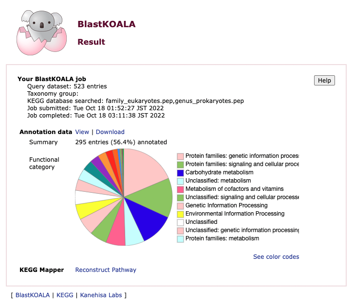
Using an annotation tool like this can help you understand more about the genes and pathways present in your sample(s). For example, as previously described, the paper this data is pulled from uses functional annotation of MAGs to look for genes associated with denitrification pathways.
Building a tree from the 16S sequence
Another option is to build a taxonomic tree to see what organisms your MAG is related to. This is possible using 16S rRNA sequences, which Prokka identifies automatically during its analysis.
Once you have an rRNA sequence you can run it through a search tool such as BLAST to find sequences which match it and what species they belong to.
We won’t be covering how to do this in detail as part of this course but you can read some instructions on how to use both BlastKOALA and BLAST towards the end of this episode of our previous Metagenomics course.
Key Points
Functional annotation allows us to look at the metabolic capacity of a metagenome
Prokka can be used to predict genes in our assembly