Taxonomic Assignment

Overview

Teaching: 30 min
Exercises: 15 min

Questions

• How can I assign a taxonomy to my raw reads?

• How can I visualise these assignments?

Objectives

• Understand how taxonomic assignment works.

• Use kraken2 to assign taxonomies to raw reads.

• Visualize taxonomic annotations in a dataset.

What is taxonomic assignment?

Taxonomic assignment is the process of assigning a sequence to a specific taxon. In this case we will be assigning our raw short reads but you can also assign metagenome-assembled genomes (MAGs), which we will be generating in next week’s lesson.

These assignments are done by comparing our sequence to a database. These searches can be done in many different ways, and against a variety of databases. There are many programs for doing taxonomic mapping, almost all of them follows one of the next strategies:

1. BLAST: Using BLAST or DIAMOND, these mappers search for the most likely hit for each sequence within a database of genomes (i.e. mapping). This strategy is slow.

2. K-mers: A genome database is broken into pieces of length k, so as to be able to search for unique pieces by taxonomic group, from lowest common ancestor (LCA), passing through phylum to species. Then, the algorithm breaks the query sequence (reads, contigs) into pieces of length k, looks for where these are placed within the tree and make the classification with the most probable position.

3. Markers: They look for markers of a database made a priori in the sequences to be classified and assign the taxonomy depending on the hits obtained.

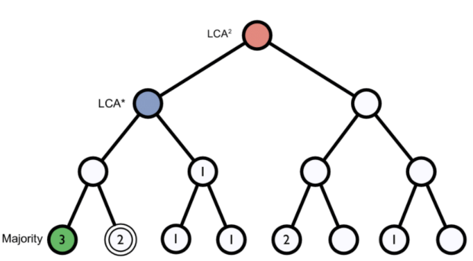
Figure 1. Lowest common ancestor assignment example.

A key result when you do taxonomic assignment of metagenomes is the abundance of each taxa in your sample. The absolute abundance of a taxon is the number of sequences (reads or contigs within a MAG, depending on how you have performed the searches) assigned to it.

We also often use relative abundance, which is the proportion of sequences assigned to it from the total number of sequences rather than absolute abundances. This is because the absolute abundance can be misleading and samples can be sequenced to different depths, and the relative abundance makes it easier to compare between samples accounting for sequencing depth differences.

It is important to be aware of the many biases that that can skew the abundances along the metagenomics workflow, shown in the figure, and that because of them we may not be obtaining the real abundance of the organisms in the sample.

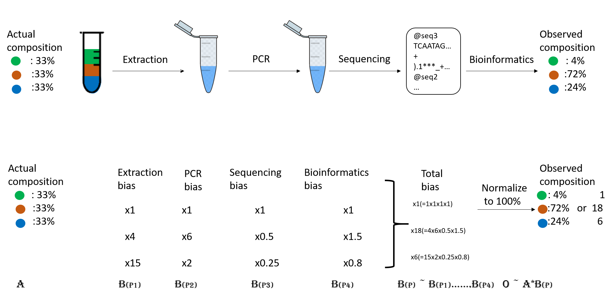Figure 2. Abundance biases during a metagenomics protocol.

Using Kraken 2

We will be using the command line program Kraken2 to do our taxonomic assignment. Kraken 2 is the newest version of Kraken, a taxonomic classification system using exact k-mer matches to achieve high accuracy and fast classification speeds.

Taxonomic assignment can be done on MAGs however we will be going back to use our raw short reads here.

kraken2 is already installed on our instance so we can look at the kraken2 help.

 kraken2  

Kraken2 help documentation

Usage: kraken2 [options] <filename(s)>

Options:
  --db NAME               Name for Kraken 2 DB
                          (default: none)
  --threads NUM           Number of threads (default: 1)
  --quick                 Quick operation (use first hit or hits)
  --unclassified-out FILENAME
                          Print unclassified sequences to filename
  --classified-out FILENAME
                          Print classified sequences to filename
  --output FILENAME       Print output to filename (default: stdout); "-" will
                          suppress normal output
  --confidence FLOAT      Confidence score threshold (default: 0.0); must be
                          in [0, 1].
  --minimum-base-quality NUM
                          Minimum base quality used in classification (def: 0,
                          only effective with FASTQ input).
  --report FILENAME       Print a report with aggregrate counts/clade to file
  --use-mpa-style         With --report, format report output like Kraken 1's
                          kraken-mpa-report
  --report-zero-counts    With --report, report counts for ALL taxa, even if
                          counts are zero
  --report-minimizer-data With --report, report minimizer and distinct minimizer
                          count information in addition to normal Kraken report
  --memory-mapping        Avoids loading database into RAM
  --paired                The filenames provided have paired-end reads
  --use-names             Print scientific names instead of just taxids
  --gzip-compressed       Input files are compressed with gzip
  --bzip2-compressed      Input files are compressed with bzip2
  --minimum-hit-groups NUM
                          Minimum number of hit groups (overlapping k-mers
                          sharing the same minimizer) needed to make a call
                          (default: 2)
  --help                  Print this message
  --version               Print version information

If none of the *-compressed flags are specified, and the filename provided
is a regular file, automatic format detection is attempted.

We will be using the flags --output and --report to specify the location of the output files Kraken will generate. And also --threads to speed up Kraken on our instance. We will also use --minimum-base-quality with a value of 30 as we are using unfiltered short reads.

In addition to our input files we also need a database (-db) with which to compare them. There are several different databases available for kraken2. Some of these are larger and much more comprehensive, and some are more specific. There are also instructions on how to generate a database of your own.

It’s very important to know your database!

The database you use will determine the result you get for your data. Imagine you are searching for a lineage that was recently discovered and it is not part of the available databases. Would you find it? Make sure you keep a note of what database you have used and when you downloaded it or when it was last updated.

You can view and download many of the common Kraken2 databases on this site. We will be using Standard-8 which is already pre installed on the instance.

Taxonomic assignment of an assembly

First, we need to make a directory for the kraken output and then we can run our kraken command.

 cd ~/cs_course/analysis/
 mkdir taxonomy

kraken2 --db ../databases/kraken_20220926/ --output taxonomy/ERR2935805.kraken --report taxonomy/ERR2935805.report --minimum-base-quality 30 --threads 8 ../data/illumina_fastq/ERR2935805.fastq

This should take around 3 - 5 minutes to run so we will run it in the foreground.

You should see an output similar to below:

Loading database information... done.
47832553 sequences (9662.18 Mbp) processed in 225.420s (12731.6 Kseq/m, 2571.78 Mbp/m).
  38990565 sequences classified (81.51%)
  8841988 sequences unclassified (18.49%)

This command generates two outputs, a .kraken and a .report file. Let’s look at the top of these files with the following commands:

head taxonomy/ERR2935805.kraken  

C	ERR2935805.1	1639	202	1637:2 0:9 1639:3 0:19 1637:8 0:17 1637:5 0:4 A:70 0:6 1637:5 0:18 1637:1 A:1
U	ERR2935805.2	0	202	A:13 286:2 A:153
U	ERR2935805.3	0	202	0:67 A:45 0:25 1637:2 A:29
U	ERR2935805.4	0	202	0:53 A:50 0:65
C	ERR2935805.5	1639	202	0:50 1639:1 0:16 A:73 0:24 1637:1 0:3
C	ERR2935805.6	1639	202	0:1 1639:5 0:3 1637:5 0:5 1637:4 0:18 1637:2 0:6 1637:5 0:13 A:35 0:17 1639:1 0:24 1637:1 0:8 1637:1 0:14
U	ERR2935805.7	0	202	A:42 0:7 A:119
C	ERR2935805.8	1639	202	0:9 1639:1 0:12 1639:1 0:23 1639:6 0:15 A:36 0:7 1639:5 0:7 1639:5 0:41
C	ERR2935805.9	1639	202	0:22 91061:5 0:9 1637:2 0:9 1637:7 0:13 A:35 0:7 1637:1 0:21 1637:3 0:8 1639:5 0:20 A:1
C	ERR2935805.10	1639	202	1639:5 0:8 1639:5 0:1 1637:2 0:36 1639:5 0:1 1639:5 0:58 1639:2 0:5 1639:1 0:13 1639:3 0:18

This gives us information about every read in the raw reads. As we can see, the kraken file is not very readable. So let’s look at the report file instead:

less taxonomy/ERR2935805.report

18.49  8841988 8841988 U       0       unclassified
 81.51  38990565        215309  R       1       root
 80.98  38733479        2279    R1      131567    cellular organisms
 80.97  38730266        124149  D       2           Bacteria
 72.67  34761467        5082    D1      1783272       Terrabacteria group
 72.64  34747831        4388    P       1239            Firmicutes
 72.63  34742819        460563  C       91061             Bacilli
 71.65  34273479        39112   O       1385                Bacillales
 70.90  33912328        1014    F       186820                Listeriaceae
 70.90  33911307        4877507 G       1637                    Listeria
 60.47  28925791        28824549        S       1639                      Listeria monocytogenes
...

Reading a Kraken report

1. Percentage of reads covered by the clade rooted at this taxon
2. Number of reads covered by the clade rooted at this taxon
3. Number of reads assigned directly to this taxon
4. A rank code, indicating (U)nclassified, (D)omain, (K)ingdom, (P)hylum, (C)lass, (O)rder, (F)amily, (G)enus, or (S)pecies. All other ranks are simply ‘-‘.
5. NCBI taxonomy ID
6. Indented scientific name

In our case, 18.49% of the reads are unclassified. These reads either didn’t meet quality threshold or were not identified in the database.

As the report is nearly 7000 lines, we will explore it with Pavian, rather than by hand.

Visualisation of taxonomic assignment results

Pavian

Pavian is a tool for the interactive visualisation of metagenomics data and allows the comparison of multiple samples. Pavian can be installed locally but we will use the browser version of Pavian.

First we need to download ERR2935805.report from our AWS instance to our local computer. Launch a git bash window or terminal which is logged into your local computer, from the cloudpan folder. Then use scp to fetch ERR2935805.report.

scp -i login-key-instanceNNN.pem csuser@instanceNNN.cloud-span.aws.york.ac.uk.:~/cs_course/analysis/taxonomy/ERR2935805.report .

Check you have included the ` .` on the end meaning copy the file ‘to here’.

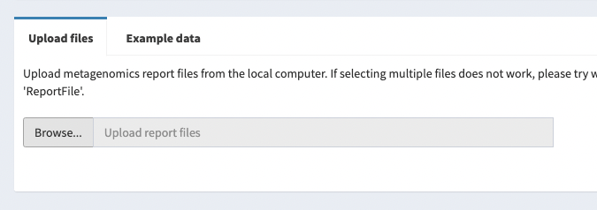
Go to Pavian site, click on Browse and upload the ERR2935805.report file you have just downloaded.

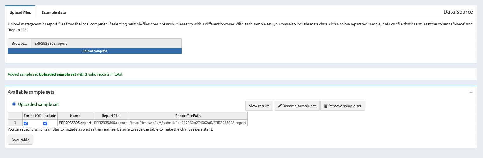
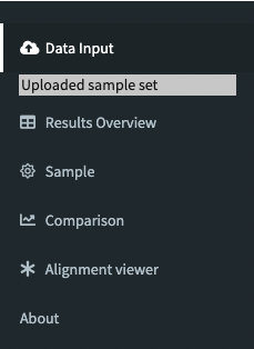
Once the file is uploaded we can explore the output generated. The column on the left has multiple different options. As we only have one sample and don’t have an alignment to view, only the “Results Overview” and “Sample” tabs are of interest to us.

At the bottom of this column there is also an option to “Generate HTML report”, this is a very good option if you wanted to share your results with others. We have used that option to generate one here for the ERR2935805 data in order to share our results. If you haven’t been able to generate a Pavian output you can view our exported example here ERR2935805-pavian-report.html (note this looks a bit different to the website version).

The Results Overview tab shows us how many reads have been classified in our sample(s). From this we can see that 18.5% of the raw reads are unclassified.

On the Sample tab we can see a Sankey diagram which shows us the proportion of our sample that has been classified at each taxa level. If you click on the “Configure Sankey” button you can play with the settings to make the diagram easier to view.

You can also view the Sankey diagram of our example here sankey-ERR2935805.report.html

Exercise 1:

Using the Sankey diagram and looking back at the information we have about our dataset are we seeing the species that we expect in our Kraken output? Are there any that we don’t expect, and if so why do you think we might be seeing them? Remember we have run this taxonomic assignment using the Standard 8GB database.

Solution

• We are seeing Listeria monocytogenes, Pseudomonas aeruginosa and Salmonella enterica in the proportions that we would expect in the Kraken output.
• We do not see Saccharomyces cerevisiae in the output, this is likely because of database choice the Standard 8GB does not contain Fungi. This is potentially why we are seeing some organisms that aren’t supposed to be in our dataset as these may be the closest approximation in this Kraken database. This is why database choice is important! You should aim to use the most comprehensive database for the compute power available to you.
• Lactobacillus fermentum has since changed it’s name to Limosilactobacillus fermentum (this is something that happens quite often with prokaryotes!) so that is also in our output.
• Less abundant organisms are harder to identify as there is just less sequencing data present for them. Bacillus subtilis, which makes up 0.89% of our dataset, has only been classified to genera level (Bacillus) as has Escherichia coli which makes up 0.089% of our dataset (Escherichia). Those with the lowest abundance Enterococcus faecalis, Cryptococcus neoformans and Staphylococcus aureus have also only been identified to a higher level.

Exercise 2: Taxonomic level of assignment

What do you think is harder to assign, a species (like E. coli) or a phylum (like Proteobacteria)?

Other software

Krona is a hierarchical data visualization software. Krona allows data to be explored with zooming, multi-layered pie charts and includes support for several bioinformatics tools and raw data formats.
Krona is used in the MG-RAST analysis pipeline which you can read more about at the end of this course.

Key Points

• Taxonomy can be assigned by comparing against a database with genome annotations. These are not exhaustive and so many things will remain unannotated depending on the samples you are analysing.

• Taxonomic assignment can be done using Kraken2.

• Pavian is a web based tool that can be used to visualize the assigned taxa.