Taxonomic Analysis with R

Overview

Teaching: 40 min
Exercises: 20 min

Questions

• How can we use standard R methods to summarise metagenomes?

• How can we plot the shared and unique compositions of samples?

• How can we compare samples with very different numbers of reads?

Objectives

• Make dataframes out of phyloseq objects

• Summarise metagenomes with standard R methods

• Make Venn diagrams for samples

• Plot absolute and relative abundances of samples

Reminder

In the last lesson, we created our phyloseq object, which contains the information of our samples: ERR2935805 and JP4D. Let´s take a look again at the number of reads in our data.

For the whole metagenome:

biom_metagenome
sample_sums(biom_metagenome)

phyloseq-class experiment-level object  
otu_table()   OTU Table:         [ 5905 taxa and 2 samples ]  
tax_table()   Taxonomy Table:    [ 5905 taxa by 7 taxonomic ranks ]  

ERR2935805       JP4D   
  38058101     149590   

Exercise 1

Repeat this for the bacterial metagenome.

Solution

Use bac_biom_metagenome instead of biom_metagenome

bac_biom_metagenome
sample_sums(bac_biom_metagenome)

phyloseq-class experiment-level object
otu_table()   OTU Table:         [ 5808 taxa and 2 samples ]
tax_table()   Taxonomy Table:    [ 5808 taxa by 7 taxonomic ranks ]

  ERR2935805       JP4D
    38057090     149590

We saw how to find out how many phlya we have and how many OTU there are in each phlya by combining commands We

• turned the tax_table into a data frame (a useful data structure in R)
• grouped by the Phylum column
• summarised by counting the number of rows for each phylum
• viewed the result This can be achieved with the following command:

bac_biom_metagenome@tax_table %>% 
  data.frame() %>% 
  group_by(Phylum) %>% 
  summarise(n = length(Phylum)) %>% 
  View()

Summarise metagenomes

phyloseq has a useful function that turns a phyloseq object into a dataframe. Since the dataframe is a standard data format in R, this makes it easier for R users to apply methods they are familiar with.

Use psmelt() to make a dataframe for the bacterial metagenomes:

bac_meta_df <- psmelt(bac_biom_metagenome)

Clicking on bac_meta_df on the Environment window will open a spreadsheet-like view of it.

Now we can more easily summarise our metagenomes by sample using standard syntax. The following filters out all the rows with zero abundance then counts the number of taxa in each phylum for each sample:

number_of_taxa <- bac_meta_df %>% 
  filter(Abundance > 0) %>% 
  group_by(Sample, Phylum) %>% 
  summarise(n = length(Abundance))

Clicking on number_of_taxa on the Environment window will open a spreadsheet-like view of it This shows us that we have some phyla:

• present in both samples such as Acidobacteria and Actinobacteria
• present in just ERR2935805 such as Candidatus Bipolaricaulota
• and present in just JP4D such as Calditrichaeota

One way to visualise the number of shared phyla is with a Venn diagram. The package ggvenn will draw one for us. It needs a data structure called a list which will contain an item for each sample of the phyla in that sample. We can see the phyla in the ERR2935805 sample with:

unique(number_of_taxa$Phylum[number_of_taxa$Sample == "ERR2935805"])

"Acidobacteria"               "Actinobacteria"              "Aquificae"                  
"Armatimonadetes"             "Bacteroidetes"               "Caldiserica"                
"Candidatus Bipolaricaulota"  "Candidatus Cloacimonetes"    "Candidatus Saccharibacteria"
"Chlamydiae"                  "Chlorobi"                    "Chloroflexi"                
"Chrysiogenetes"              "Cyanobacteria"               "Deferribacteres"            
"Deinococcus-Thermus"         "Elusimicrobia"               "Firmicutes"                 
"Fusobacteria"                "Gemmatimonadetes"            "Kiritimatiellaeota"         
"Nitrospirae"                 "Planctomycetes"              "Proteobacteria"             
"Spirochaetes"                "Synergistetes"               "Tenericutes"                
"Thermodesulfobacteria"       "Thermotogae"                 "Verrucomicrobia"

Exercise 2

Repeat this for the JP4D sample

Solution

Use JP4D instead of ERR2935805

unique(number_of_taxa$Phylum[number_of_taxa$Sample == "JP4D"])

"Acidobacteria"               "Actinobacteria"              "Aquificae"                  
"Armatimonadetes"             "Bacteroidetes"               "Caldiserica"                
"Calditrichaeota"             "Candidatus Cloacimonetes"    "Candidatus Saccharibacteria"
"Chlamydiae"                  "Chlorobi"                    "Chloroflexi"                
"Chrysiogenetes"              "Coprothermobacterota"        "Cyanobacteria"              
"Deferribacteres"             "Deinococcus-Thermus"         "Dictyoglomi"                
"Elusimicrobia"               "Fibrobacteres"               "Firmicutes"                 
"Fusobacteria"                "Gemmatimonadetes"            "Ignavibacteriae"            
"Kiritimatiellaeota"          "Lentisphaerae"               "Nitrospirae"                
"Planctomycetes"              "Proteobacteria"              "Spirochaetes"               
"Synergistetes"               "Tenericutes"                 "Thermodesulfobacteria"      
"Thermotogae"                 "Verrucomicrobia"      

To place the two sets of phlya in a list, we use

venn_data <- list(ERR2935805 = unique(number_of_taxa$Phylum[number_of_taxa$Sample == "ERR2935805"]),
                  JP4D = unique(number_of_taxa$Phylum[number_of_taxa$Sample == "JP4D"]))

And to draw the venn diagram

ggvenn(venn_data)

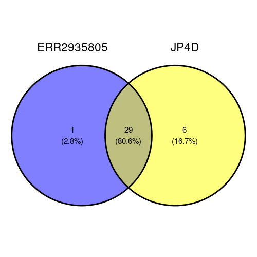The Venn diagram shows that most of the phyla (29 which is 80.6%) are in both samples, one is in ERR2935805 only and 6 are in JP4D only. Perhaps you would like to know which phyla is in ERR2935805 only? The following command will print that for us:

venn_data$ERR2935805[!venn_data$ERR2935805 %in% venn_data$JP4D]

"Candidatus Bipolaricaulota"

Exercise 3

Which phyla are in JP4D only?

Solution

Use JP4D instead of ERR2935805 and ERR2935805 instead of JP4D!

venn_data$JP4D[!venn_data$JP4D %in% venn_data$ERR2935805]

"Calditrichaeota"      "Coprothermobacterota" "Dictyoglomi"         
"Fibrobacteres"        "Ignavibacteriae"      "Lentisphaerae"  

We summarised our metagenomes for the number of phyla in each sample in number_of_taxa. We can use a similar approach to examine the abundance of each of these taxa:

abundance_of_taxa <- bac_meta_df %>% 
  filter(Abundance > 0) %>% 
  group_by(Sample, Phylum) %>% 
  summarise(Abundance = sum(Abundance))

We can see the vast majority of our taxa are Proteobacteria and Firmicutes in ERR2935805

Visualizing our data

It would be nice to see the abundance by tax as a figure. We can use the ggplot() function to visualise the breakdown by Phylum in each of our two bacterial metagenomes:

abundance_of_taxa %>% 
  ggplot(aes(x = Sample, y = Abundance, fill = Phylum)) +
  geom_col(position = "stack")

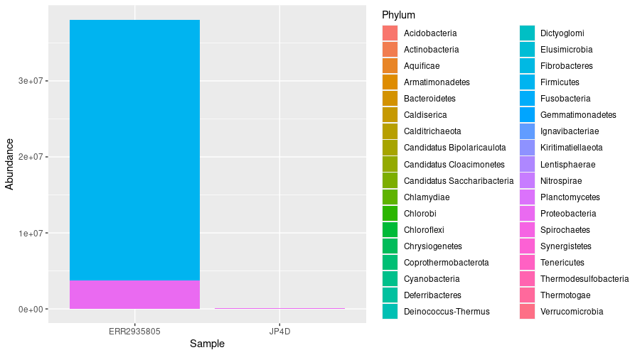
We can see that the most abundant phyla in ERR2935805 are Proteobacteria and Firmicutes. However, we can’t tell much from JP4D because the total number of reds is so much less.

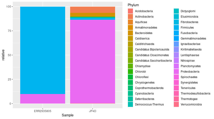
Transformation of data

Since our metagenomes have different sizes, it is imperative to convert the number of assigned read into percentages (i.e. relative abundances) to compare them.

We can achieve this with:

abundance_of_taxa <- abundance_of_taxa %>% 
  group_by(Sample) %>% 
  mutate(relative = Abundance/sum(Abundance) * 100)

Then plot the result:

abundance_of_taxa %>% 
  ggplot(aes(x = Sample, y = relative, fill = Phylum)) +
  geom_col(position = "stack")

Key Points

• The R package phyloseq has a function psmelt() to make dataframes from phyloseq objects.

• A venn diagram can be used to show the shared and unique compositions of samples.

• Plotting relative abundance allows you to compare samples with differing numbers of reads