Diversity Tackled With R
Overview
Teaching: 40 min
Exercises: 10 minQuestions
What are α and β diversity? What are the metrics used to measure these?
How can I obtain the abundance of the reads?
How can I use R to explore diversity?
Objectives
Explain α and β diversity.
Explain what a BIOM table is and be able to generate one with
kraken-biomUse R to summarise metagenomes and calculate diversity indices.
Once we know the taxonomic composition of our metagenomic sequencing data we can characterise them by their diversity. In this episode we will first define what we mean by diversity and then calculate the α diversity in our sample. We will also calculate the diversity of another sample.
What is diversity?
Species diversity is the number of species in a system and the relative abundance of each of those species. It can be defined on three different scales (Whittaker, 1960).
- the total species diversity in an ecosystem known as gamma (γ) diversity
- average diversity at a local site, known as alpha (α) diversity
- the difference in diversity between local sites, known as beta (β) diversity
A metagenome can be considered a local site. In this episode we will calculate α diversity (that within a metagenome) and β diversity (that between metagenomes).
Alpha (α) diversity
The simplest measure of α diversity is the number of species, or species richness. However, most indices of α diversity take into account both the number of species and their relative abundances, or species evenness. Different diversity indices weight these two components differently.
| α Diversity Index | Description | Calculation | Where |
|---|---|---|---|
| Shannon (H) | Estimation of species richness and species evenness. More weight on richness. | \(H = - \sum_{i=1}^{S} p_{i} \ln{p_{i}}\) | \(S\) is the number of OTUs and \(p_{i}\) is the proportion of the community represented by OTU |
| Simpson’s (D) | Estimation of species richness and species evenness. More weight on evenness. | \(D = \frac{1}{\sum_{i=1}^{S} p_{i}^{2}}\) | \(S\) is Total number of the species in the community and \(p_{i}\) is the proportion of community represented by OTU i |
| Chao1 | Abundance based on species represented by a single individual (singletons) and two individuals (doubletons). | \(S_{chao1} = S_{Obs} + \frac{F_{1} \times (F_{1} - 1)}{2 \times (F_{2} + 1)}\) | \(F_{1}\) and \(F_{2}\) are the counts of singletons and doubletons respectively and \(S_{chao1}=S_{Obs}\) is the number of observed species |
 Figure 1. Alpha diversity represented by fish in a pond. Here, alpha diversity is measured in the simplest way using species richness.
Beta (β) diversity
β diversity measures how different two or more communities are in their richness, evenness or both.
| β Diversity Index | Description |
|---|---|
| Bray–Curtis dissimilarity | The compositional dissimilarity between two metagenomes, based on counts in each metagenome. Ranges from 0 (the two metagenomes have the same species composition) to 1 (the two metagenomes do not share any species). Bray–Curtis dissimilarity emphasises abundance. |
| Jaccard distance | Also ranges from 0 (the two metagenomes have the same species) to 1 (the two metagenomes do not share any species) but is based on the presence or absence of species only. This means it emphasises richness. |
| UniFrac | Differs from the Bray-Curtis dissimilarity and Jaccard distance by including the relatedness between taxa in a metagenome. Measures the phylogenetic distance between metagenomes as the proportion of unshared phylogenetic tree branches. Weighted-Unifrac takes into account the relative abundance of taxa shared between samples; unweighted-Unifrac only considers presence or absence. |
Figure 2 shows α and the β diversity for three lakes. The most simple way to calculate the β diversity is to calculate the number of species that are unique in two lakes. For example, the number of species in Lake A (the α diversity) is 3 and 1 of these is also found in Lake C; the number of species in Lake C is 2 and 1 of these is also in Lake A. The β diversity between A and C is calculated as (3 - 1) + (2 - 1) = 3
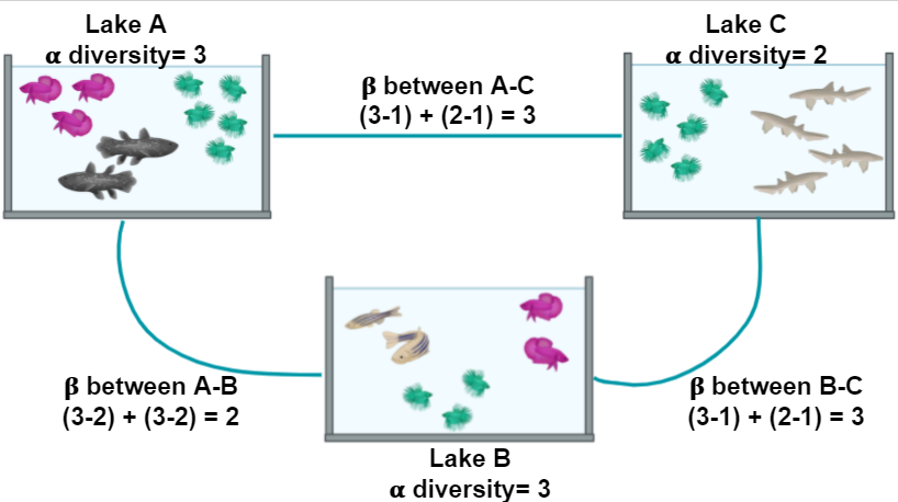 Figure 2. Alpha and Beta diversity represented by fishes in a pond.
Exercise 1:
In the next picture there are two lakes with different fish species:
Which of the options below is true:
- α diversity of A = 4, α diversity of B = 3, β diversity between A and B = 1
- α diversity of A = 4, α diversity of B = 3, β diversity between A and B = 5
- α diversity of A = 9, α diversity of B = 7, β diversity between A and B= 16
Please, paste your result on the collaborative document provided by instructors.
Solution
Answer: 2. α diversity of A = 4, α diversity of B = 3, β diversity between A and B = 5 The number of species in Lake A (the α diversity) is 4 and 1 of these is also found in Lake B; the number of species in Lake B is 3 and 1 of these is also in Lake A. The β diversity between A and C is calculated as (4 - 1) + (3 - 1) = 5.
How do we calculate diversity from metagenomic samples?
We will calculate the diversity in our heathland sample ERR4998593 and compare it with data from another site from the same study: ERR4998600. This is a fenland site (so lower and wetter than our heathland site).
There are 2 steps needed to calculate the diversity of our samples.
- Create a Biological Observation Matrix, BIOM table, from the Kraken output. A BIOM table is a matrix of counts with samples in the columns and taxa in the rows. The values in the matrix are the counts of that taxa in that sample.
- Analyse the BIOM table to generate diversity indices and relative abundance plots.
What part of the Kraken output do we need?
We will use a command-line program called kraken-biom to convert our Kraken output into a BIOM table. kraken-biom takes the .report output of Kraken and creates a BIOM table in .biom format.
Move in to your taxonomy folder
cd ~/cs_course/analysis/taxonomy
List the files
ls -l
-rw-rw-r-- 1 csuser csuser 3935007137 Apr  9 09:16 ERR4998593.kraken
-rw-rw-r-- 1 csuser csuser     424101 Apr  9 09:16 ERR4998593.report
As we saw in the previous episode, .kraken and .report are the output files generated by Kraken.
We will also need the ERR4998600 Kraken report. We have put this in our GitHub repo and it can be copied into your taxonomy directory on the instance using wget. This is a useful command for retrieving files from web servers and simply requires wget followed by the web address the file is stored at.
wget https://cloud-span.github.io/nerc-metagenomics06-taxonomic-anno/files/ERR4998600.report
You should ls to check that this file has been downloaded.
Create the BIOM table
kraken-biom has many options which you can see with the help command. However, we only need to specify an output format --fmt of json to use the file in the next step.
kraken-biom -houtputusage: kraken-biom [-h] [--max {D,P,C,O,F,G,S}] [--min {D,P,C,O,F,G,S}] [-o OUTPUT_FP] [--otu_fp OTU_FP] [--fmt {hdf5,json,tsv}] [--gzip] [--version] [-v] kraken_reports [kraken_reports ...] Set the output format of the BIOM table. Default is HDF5. Create BIOM-format tables (http://biom-format.org) from Kraken output BIOM (v2.x) files are internally compressed by default, so this option is not needed when (http://ccb.jhu.edu/software/kraken/).mt hdf5. --version show program's version number and exit The program takes as input, one or more files output from the kraken-report tool. Each file is parsed and the counts for each OTU (operational taxonomic unit) are recorded, along with database ID (e.g. NCBI), and lineage. The extracted data are then stored in a BIOM table where each count is linked to the Sample and OTU it belongs to. Sample IDs are extracted from the input filenames (everything up to the '.'). OTUs are defined by the --max and --min arguments. By default these are set to Order and Species respectively. This means that counts assigned directly to an Order, Family, or Genus are recorded under the associated OTU ID, and counts assigned at or below the Species level are assigned to the OTU ID for the species. Setting a minimum rank below Species is not yet available. The BIOM format currently has two major versions. Version 1.0 uses the JSON (JavaScript Object Notation) format as a base. Version 2.x uses the HDF5 (Hierarchical Data Format v5) as a base. The output format can be specified with the --fmt option. Note that a tab-separated (tsv) output format is also available. The resulting file will not contain most of the metadata, but can be opened by spreadsheet programs. Version 2 of the BIOM format is used by default for output, but requires the Python library 'h5py'. If the library is not installed, kraken-biom will automatically switch to using version 1.0. Note that the output can optionally be compressed with gzip (--gzip) for version 1.0 and TSV files. Version 2 files are automatically compressed. Usage examples -------------- 1. Basic usage with default parameters: $ kraken-biom.py S1.txt S2.txt This produces a compressed BIOM 2.1 file: table.biom 2. BIOM v1.0 output: $ kraken-biom.py S1.txt S2.txt --fmt json Produces a BIOM 1.0 file: table.biom 3. Compressed TSV output: $ kraken-biom.py S1.txt S2.txt --fmt tsv --gzip -o table.tsv Produces a TSV file: table.tsv.gz 4. Change the max and min OTU levels to Class and Genus: $ kraken-biom.py S1.txt S2.txt --max C --min G Program arguments ----------------- positional arguments: kraken_reports Results files from the kraken-report tool. optional arguments: -h, --help show this help message and exit --max {D,P,C,O,F,G,S} Assigned reads will be recorded only if they are at or below max rank. Default: O. --min {D,P,C,O,F,G,S} Reads assigned at and below min rank will be recorded as being assigned to the min rank level. Default: S. -o OUTPUT_FP, --output_fp OUTPUT_FP Path to the BIOM-format file. By default, the table will be in the HDF5 BIOM 2.x format. Users can output to a different format using the --fmt option. The output can also be gzipped using the --gzip option. Default path is: ./table.biom --otu_fp OTU_FP Create a file containing just the (NCBI) OTU IDs for use with a service such as phyloT (http://phylot.biobyte.de/) to generate a phylogenetic tree for use in downstream analysis such as UniFrac, iTol (itol.embl.de), or PhyloToAST (phylotoast.org). --fmt {hdf5,json,tsv} Set the output format of the BIOM table. Default is HDF5. --gzip Compress the output BIOM table with gzip. HDF5 BIOM (v2.x) files are internally compressed by default, so this option is not needed when specifying --fmt hdf5. --version show program's version number and exit -v, --verbose Prints status messages during program execution.
With the next command, we are going to create a table in Biom format from our two Kraken reports: ERR4998593.report and ERR4998600.report.
We customise the command with a couple of flags:
--fmt jsontells kraken-biom that we want the output table to be in JSON format as opposed to the default HDF5 BIOM2.x format-o metagenome.biommeans our output table will be namedmetagenome.biom
kraken-biom ERR4998593.report ERR4998600.report --fmt json -o metagenome.biom
kraken-biom uses both reports to generate the BIOM table. The BIOM table is in a file called metagenome.biom.
ls -l
-rw-rw-r-- 1 csuser csuser 3935007137 Apr  9 09:16 ERR4998593.kraken
-rw-rw-r-- 1 csuser csuser     424101 Apr  9 09:16 ERR4998593.report
-rw-rw-r-- 1 csuser csuser     404232 Apr  9 09:30 ERR4998600.report
-rw-rw-r-- 1 csuser csuser     741259 Apr  9 10:22 metagenome.biom
Analyse the BIOM table using R
We will be using an R package called phyloseq to analyse our biom file. Other software for analyses of diversity include Qiime2, MEGAN and the R package Vegan
If you are very familiar with R and RStudio and already have them on your machine, you may want to install the packages needed and download the metagenome.biom file to do the analysis on your own computer. However, you do not need prior experience with R and RStudio for this part of the course: we have set up the analysis in RStudio Cloud, an online version of RStudio which has everything you need, including the code. We have given instructions for both options.
Option A: I know R and RStudio.
If you know R and RStudio and already have them on your machine you may want to use this option.
- Open RStudio
- Install the packages
You will needphyloseq, a Bioconductor package, and thetidyverseandggvennpackages. Bioconductor packages are installed using theinstall()function from theBioManagerpackage so we first install that, thenphyloseq,tidyverseandggvenn:> install.packages("BiocManager") > BiocManager::install("phyloseq") > install.packages("tidyverse") > install.packages("ggvenn") - Make an RStudio project
Make an RStudio project workshop by clicking on the drop-down menu on top right where it says Project: (None) and choosing New Project and then New Directory, then New Project. In the “Create project as a subdirectory” box, use Browse to navigate to the “cloudspan” folder. Name the RStudio Project ‘diversity’. - Download the
metagenome.biomfile to the project folder
Download the file to the project folder usingscp. Use a terminal that is not logged into the cloud instance and ensure you are in yourcloudspandirectory. Usescpto copy the file to thediversityfolder - the command will look something like:scp -i login-key-instanceNNN.pem csuser@instanceNNN.cloud-span.aws.york.ac.uk:~/cs_course/analysis/taxonomy/metagenome.biom diversityRemember to replace NNN with the instance number specific to you.
- Open a new script.
Now go to Start the analysis.
Option B: I don’t know R and RStudio.
If you don’t know R and RStudio we suggest you to use this option. We have installed the packages needed and put the data, metagenome.biom and a script analysis.R in the RStudio Cloud Project.
- Make an RStudio Cloud account
Go to https://rstudio.cloud/ and follow Get Started for Free. We recommend signing up with your Google account if you use one. - Follow the link to the cloud-span-metagenomics project.
Open the project we have set up: cloud-span-metagenomics. You’ll get a message saying “Deploying project”. This will take a few seconds. - Open
analysis.Rfrom the Files pane on the bottom right of the display.
Start the Analysis
If you are using RStudio Cloud, we will run through the code in analysis.R line by line. If you are using RStudio on your own machine you can type in the commands or copy them from analysis.R
First load the packages we need. Put your cursor on the line you want to run and press CTRLENTER
library("phyloseq")
library("tidyverse")
library("ggvenn")
Now import the data in metagenome.biom into R using the import_biom() function from phyloseq
biom_metagenome <- import_biom("metagenome.biom")
This command produces no output in the console but created a special class of R object which is defined by the phyloseq package and called it biom_metagenome. Click on the object name, biom_metagenome, in the Environment pane (top right), see the screenshot below. This will open a view of the object in the same pane as your script.
A phyloseq object is a special object in R. It has five parts, called ‘slots’ which you can see listed in the object view. These are otu_table, tax_table, sam_data, phy_tree and refseq. In our case, sam_data, phy_tree and refseq are empty. The useful data are in otu_table and tax_table`.

Return to your script (click on the tab). Typing biom_metagenome will give some summary information about the biom_metagenome object:
biom_metagenome
phyloseq-class experiment-level object
otu_table()   OTU Table:         [ 7637 taxa and 2 samples ]
tax_table()   Taxonomy Table:    [ 7637 taxa by 7 taxonomic ranks ]
The line starting otu_table tells us we have two samples - these are ERR4998593 and ERR4998600 - with a total of 7637 taxa. The tax_table again tells us how many taxa we have. The seven ranks indicates that we have some identifications down to species level. The taxonomic ranks are from the classification system of taxa from the most general (kingdom) to the most specific (species): kingdom/domain, phylum, class, order, family, genus, species.
We can view the tax_table with:
View(biom_metagenome@tax_table)
This table has the OTU identity in the row names and the samples in the columns. The values in the columns are the abundance of that OTU in that sample.
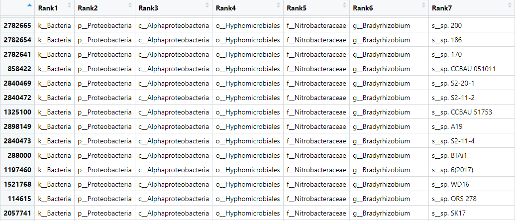 Figure 3. Table of the OTU data from our
 biom_metagenome object.
To make downstream analysis easier for us we will remove the prefix (e.g. f__) on each item. This contains information about the rank of the assigned taxonomy, we don’t want to lose this information so will and instead rename the header of each column of the DataFrame to contain this information.
To remove unnecessary characters we are going to use command substring().
This command is useful to extract or replace characters in a vector. To use the command, we have to indicate the vector (x) followed by the first element to replace or extract (first) and the last element to be replaced (last). For instance: substring (x, first, last). If a last position is not used it will be set to the end of the string.
The prefix for each item in biom_metagenome is made up of a letter and two underscores, for example: o__Bacillales. In this case “Bacillales” starts at position 4 with a B.
So to remove the unnecessary characters we will use the following code:
biom_metagenome@tax_table <- substring(biom_metagenome@tax_table, 4)
Let’s change the names of the columns too:
colnames(biom_metagenome@tax_table) <- c("Kingdom",
           "Phylum",
           "Class",
           "Order",
           "Family",
           "Genus",
           "Species")
Check it worked:
View(biom_metagenome@tax_table)
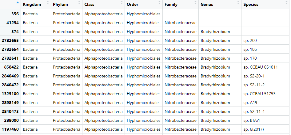 Figure 4. Table of the OTU data from our
 biom_metagenome object. With corrections.
How many OTUs are in each kingdom? We can find out by combining some commands. We need to:
- turn the tax_table into a data frame (a useful data structure in R)
- group by the Kingdom column
- summarise by counting the number of rows for each Kingdom
This can be achieved with the following command:
biom_metagenome@tax_table %>%
  data.frame() %>%
  group_by(Kingdom) %>%
  summarise(n = length(Kingdom))
# A tibble: 4 × 2
  Kingdom       n
  <chr>     <int>
1 Archaea     339
2 Bacteria   7231
3 Eukaryota     1
4 Viruses      66
Most things are bacteria!
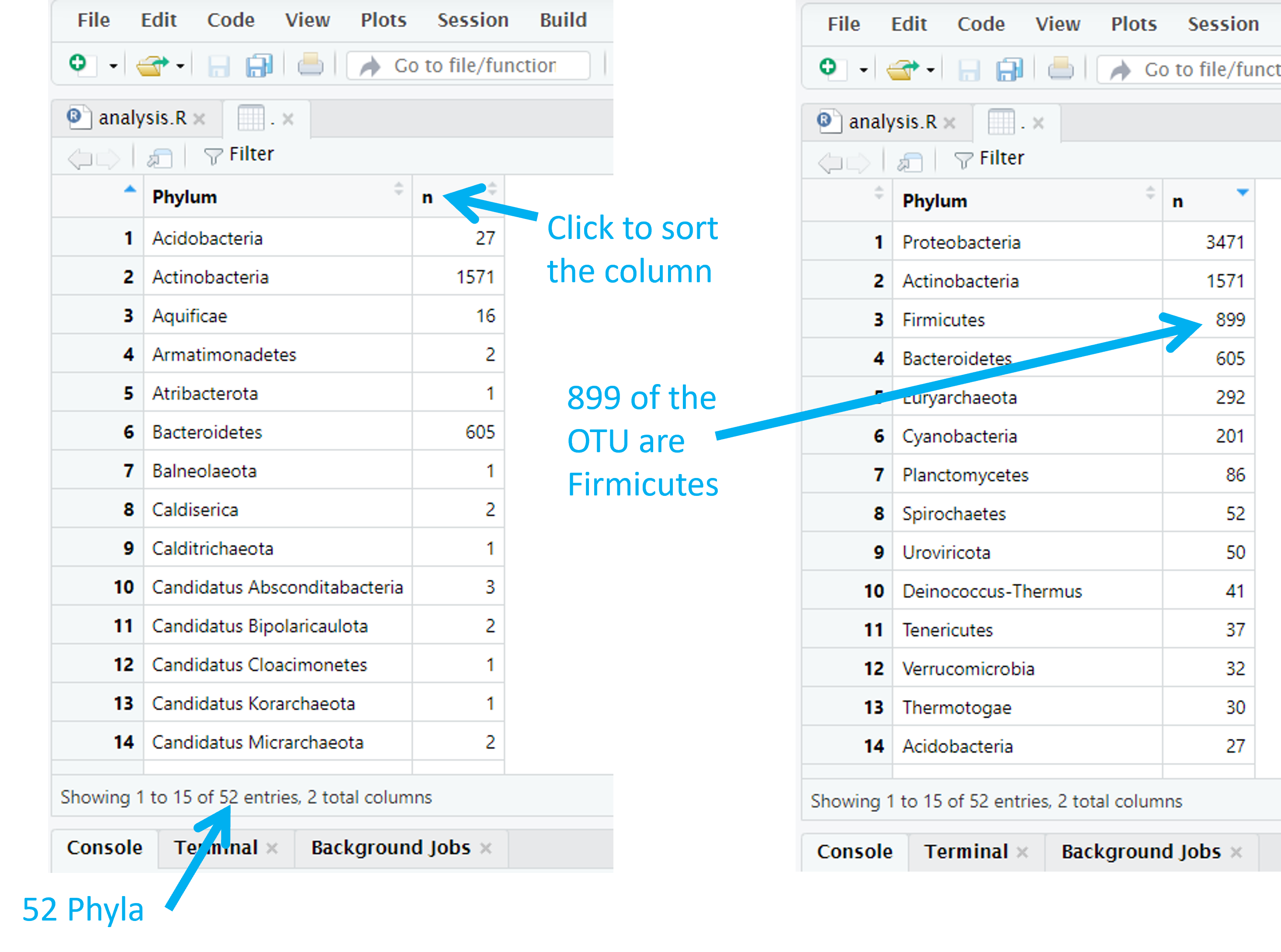
We can explore how many phlya we have and how many OTU there are in each phlya in a similar way. This time we will use View() to see the whole table because it won’t all print to the console
- turn the tax_table into a data frame (a useful data structure in R)
- group by the Phylum column
- summarise by counting the number of rows for each phylum
- viewing the result
This can be achieved with the following command:
biom_metagenome@tax_table %>%
 data.frame() %>%
 group_by(Phylum) %>%
 summarise(n = length(Phylum)) %>%
 View()
This shows us a table with a phylum, and the number times it appeared, in each row. The number of phyla is given by the number of rows in this table. By defualt, the table is sorted alphabetically by phylum. We can sort by frequency by clicking on the ‘n’ column. There are 3471 Proteobacteria and 1571 Actinobacteria for example.
Exercise 2: Explore the Orders
Adapt the code to explore how many Orders we have and how many OTU there are in each order.
a) How many orders are there?
b) What is the most common order?
c) How many OTUs did not get down to order level?Solution
You should the use the column name ‘Order’ instead of ‘Phylum’ in the code
biom_metagenome@tax_table %>%
  data.frame() %>%
  group_by(Order) %>%
  summarise(n = length(Order)) %>%
  View()
a) 229. This is the number of rows in the table
b) Hyphomicrobiales. Sorting the column n will bring this to the top. Hyphomicrobiales appears 480 times
c) 66. If an OTU has not been identified to order level the order column will be blank. The table shows there were 66 such cases (you can find this more easily by sorting the column Order).
Plot alpha diversity
We want to explore the bacterial diversity of our samples, so we will remove all of the non-bacterial organisms. To do this we will generate a subset of all bacterial groups and save them.
bac_biom_metagenome <- subset_taxa(biom_metagenome, Kingdom == "Bacteria")
Now let’s look at some statistics of our bacterial metagenomes:
bac_biom_metagenome
phyloseq-class experiment-level object
otu_table()   OTU Table:         [ 7231 taxa and 2 samples ]
tax_table()   Taxonomy Table:    [ 7231 taxa by 7 taxonomic ranks ]
phyloseq includes a function to find the sample names and one to count the number of reads in each sample.
Find the sample names with sample_names():
sample_names(bac_biom_metagenome)
"ERR4998593" "ERR4998600"
Count the number of reads with sample_sums():
sample_sums(bac_biom_metagenome)
ERR4998593 ERR4998600
    442490     305135
The summary() function can give us an indication of species evenness
summary(bac_biom_metagenome@otu_table)
 ERR4998593         ERR4998600
Min.   :    0.00   Min.   :    0.0
1st Qu.:    1.00   1st Qu.:    2.0
Median :    6.00   Median :   11.0
Mean   :   61.19   Mean   :   42.2
3rd Qu.:   31.50   3rd Qu.:   38.0
Max.   :60679.00   Max.   :38768.0
The median in sample ERR4998593 is 6, meaning many of OTU occur six times. The maximum is very high so at least one OTU is very abundant.
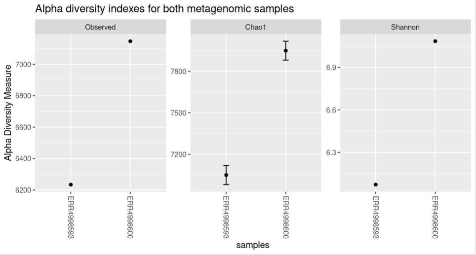
The plot_richness() command will give us a visual representation of the diversity inside the samples (i.e. α diversity):
plot_richness(physeq = biom_metagenome,
              measures = c("Observed","Chao1","Shannon"))
 Figure 5. Alpha diversity indexes for both samples.
Each of these metrics can give insight of the distribution of the OTUs inside our samples. For example Chao1 diversity index gives more weight to singletons and doubletons observed in our samples, while the Shannon is a measure of species richness and species evenness with more weigth on richness.
Use the following to open the manual page for plot_richness
?plot_richness
Exercise 3:
While using the help provided explore these options available for the function in
plot_richness():
nrowsortbytitleUse these options to generate new figures that show you other ways to present the data.
Solution
The code and the plot using the three options will look as follows: The “title” option adds a title to the figure.
plot_richness(physeq = biom_metagenome,
             title = "Alpha diversity indexes for both metagenomic samples",
             measures = c("Observed","Chao1","Shannon"))
The “nrow” option arranges the graphics horizontally.
plot_richness(physeq = biom_metagenome,
             title = "Alpha diversity indexes for both metagenomic samples",
             measures = c("Observed","Chao1","Shannon"),
             nrow=3)
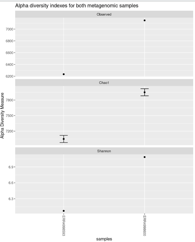
The “sortby” option orders the samples from least to greatest diversity depending on the parameter. In this case, it is ordered by “Shannon” and tells us that the ERR4998593 sample has the lowest diversity and the ERR4998600 sample the highest.
plot_richness(physeq = bac_biom_metagenome,
             title = "Alpha diversity indexes for both metagenomic samples",
             measures = c("Observed","Chao1","Shannon"),
             sortby = "Shannon")

Beta diversity
The β diversity between ERR4998593 and ERR4998600 can be calculated with the distance() function. For example, we can
find the Bray–Curtis dissimilarity with:
distance(bac_biom_metagenome, method="bray")
           ERR4998593
ERR4998600  0.5438328
There are other methods of determining distance and we can view our options with:
distanceMethodList$vegdist
[1] "manhattan"  "euclidean"  "canberra"   "bray"       "kulczynski" "jaccard"    "gower"
[8] "altGower"   "morisita"   "horn"       "mountford"  "raup"       "binomial"   "chao"
[15] "cao"
Any of these methods can be used in the same way used above, e.g.
distance(bac_biom_metagenome, method="jaccard")
           ERR4998593
ERR4998600  0.7045229
The output of this function is a distance matrix. When we have just two samples there is only one distance to calculate. If we had many samples, the output would have the pairwise distances between all of them
Reading
Tuomisto, H. A consistent terminology for quantifying species diversity? Yes, it does exist. Oecologia 164, 853–860 (2010). https://doi.org/10.1007/s00442-010-1812-0
Whittaker, R. H. (1960) Vegetation of the Siskiyou Mountains, Oregon and California. Ecological Monographs, 30, 279–338
Key Points
α diversity measures diversity in a metagenome
β diversity measures the difference in diversity between metagenomes.
A Biological Observation Matrix, BIOM table is a matrix of counts and is generated from the Kraken output using
kraken-biomThe
phyloseqpackage can be used to analyse metagenome diversity using the BIOM table.