Taxonomic Assignment
Overview
Teaching: 30 min
Exercises: 15 minQuestions
How can I assign a taxonomy to my raw reads?
How can I visualise these assignments?
Objectives
Understand how taxonomic assignment works.
Use kraken2 to assign taxonomies to raw reads.
Visualize taxonomic annotations in a dataset.
What is taxonomic assignment?
Taxonomic assignment is the process of assigning a sequence to a specific taxon. In this case we will be assigning our raw short reads but you can also assign metagenome-assembled genomes (MAGs).
We are using short reads rather than MAGs because we want to look at the relative differences in abundance between the taxa. This would be much less accurate using MAGs since these are compilations of fragments.
These assignments are done by comparing our sequence to a database. These searches can be done in many different ways, and against a variety of databases. There are many programs for doing taxonomic mapping; almost all of them follows one of these strategies:
-
BLAST: Using BLAST or DIAMOND, these mappers search for the most likely hit for each sequence within a database of genomes (i.e. mapping). This strategy is slow.
-
K-mers: A genome database is broken into pieces of length k, so as to be able to search for unique pieces by taxonomic group, from lowest common ancestor (LCA), passing through phylum to species. Then, the algorithm breaks the query sequence (reads, contigs) into pieces of length k, looks for where these are placed within the tree and make the classification with the most probable position.
-
Markers: This method looks for markers of a database made a priori in the sequences to be classified and assigns the taxonomy depending on the hits obtained.
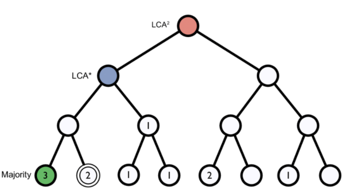
Figure 1. Lowest common ancestor assignment example.
A key result when you do taxonomic assignment of metagenomes is the abundance of each taxa in your sample. The absolute abundance of a taxon is the number of sequences (reads or contigs within a MAG, depending on how you have performed the searches) assigned to it.
We also often use relative abundance, which is the proportion of sequences assigned to it from the total number of sequences rather than absolute abundances. This is because the absolute abundance can be misleading and samples can be sequenced to different depths, and the relative abundance makes it easier to compare between samples accounting for sequencing depth differences.
It is important to be aware of the many biases that that can skew the abundances along the metagenomics workflow, shown in the figure, and that because of them we may not be obtaining the real abundance of the organisms in the sample.
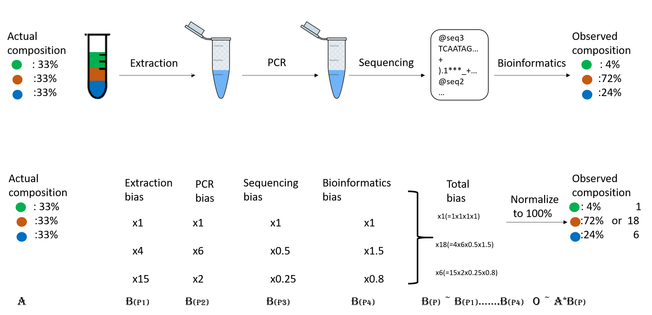 Figure 2. Abundance biases during a metagenomics protocol.
Using Kraken 2
We will be using the command line program Kraken2 to do our taxonomic assignment. Kraken 2 is the newest version of Kraken, a taxonomic classification system using exact k-mer matches to achieve high accuracy and fast classification speeds.
Taxonomic assignment can be done on MAGs however we will be going back to use our raw short reads here.
kraken2 is already installed on our instance so we can look at the kraken2 help.
kraken2
Kraken2 help documentation
Usage: kraken2 [options] <filename(s)>

Options:
  --db NAME               Name for Kraken 2 DB
                          (default: none)
  --threads NUM           Number of threads (default: 1)
  --quick                 Quick operation (use first hit or hits)
  --unclassified-out FILENAME
                          Print unclassified sequences to filename
  --classified-out FILENAME
                          Print classified sequences to filename
  --output FILENAME       Print output to filename (default: stdout); "-" will
                          suppress normal output
  --confidence FLOAT      Confidence score threshold (default: 0.0); must be
                          in [0, 1].
  --minimum-base-quality NUM
                          Minimum base quality used in classification (def: 0,
                          only effective with FASTQ input).
  --report FILENAME       Print a report with aggregrate counts/clade to file
  --use-mpa-style         With --report, format report output like Kraken 1's
                          kraken-mpa-report
  --report-zero-counts    With --report, report counts for ALL taxa, even if
                          counts are zero
  --report-minimizer-data With --report, report minimizer and distinct minimizer
                          count information in addition to normal Kraken report
  --memory-mapping        Avoids loading database into RAM
  --paired                The filenames provided have paired-end reads
  --use-names             Print scientific names instead of just taxids
  --gzip-compressed       Input files are compressed with gzip
  --bzip2-compressed      Input files are compressed with bzip2
  --minimum-hit-groups NUM
                          Minimum number of hit groups (overlapping k-mers
                          sharing the same minimizer) needed to make a call
                          (default: 2)
  --help                  Print this message
  --version               Print version information

If none of the *-compressed flags are specified, and the filename provided
is a regular file, automatic format detection is attempted.
In addition to our input files we will need a database (-db) with which to compare them. There are several different databases available for kraken2. Some of these are larger and much more comprehensive, and some are more specific. There are also instructions on how to generate a database of your own.
It’s very important to know your database!
The database you use will determine the result you get for your data. Imagine you are searching for a lineage that was recently discovered and it is not part of the available databases. Would you find it? Make sure you keep a note of what database you have used and when you downloaded it or when it was last updated.
You can view and download many of the common Kraken2 databases on this site. We will be using Standard-8 which is already pre installed on the instance.
Taxonomic assignment of an assembly
First, we need to make a directory for the kraken output and then we can run our kraken command.
We use the following flags:
--outputto specify the location of the.krakenoutput file--reportto specify the location of the.reportoutput file--threadsto specify the number of threads to use--minimum-base-qualityto exclude bases with a PHRED quality score below a certain threshold (most important if you haven’t filtered your short reads)--dbto tell Kraken2 where to find the database to compare the reads to
 cd ~/cs_course/analysis/
 mkdir taxonomy

kraken2 --db ../databases/kraken_20220926/ --output taxonomy/ERR4998593.kraken --report taxonomy/ERR4998593.report --minimum-base-quality 30 --threads 8 ../data/illumina_fastq/ERR4998593_1.fastq ../data/illumina_fastq/ERR4998593_2.fastq
This should take around 3 - 5 minutes to run so we will run it in the foreground.
You should see an output similar to below:
Loading database information... done.
68527220 sequences (10347.61 Mbp) processed in 109.270s (37628.2 Kseq/m, 5681.86 Mbp/m).
  616037 sequences classified (0.90%)
  67911183 sequences unclassified (99.10%)
This command generates two outputs, a .kraken and a .report file. Let’s look at the top of these files with the following command:
head taxonomy/ERR4998593.kraken
U       ERR4998593.40838091     0       151     A:117
U       ERR4998593.57624042     0       151     0:113 A:4
U       ERR4998593.3    0       151     A:1 0:39 A:34 0:43
U       ERR4998593.4    0       151     A:1 0:8 A:34 0:73 A:1
U       ERR4998593.34339006     0       151     A:20 0:41 A:56
U       ERR4998593.6    0       151     A:1 0:17 A:99
U       ERR4998593.59019952     0       151     A:117
C       ERR4998593.34862640     2686094 151     0:9 A:62 0:6 2686094:5 0:10 28211:1 0:24
U       ERR4998593.63611176     0       151     0:1 A:42 0:58 A:16
U       ERR4998593.57807180     0       151     A:5 0:112
This gives us information about every read in the raw reads. As we can see, the kraken file is not very readable. So let’s look at the report file instead:
less taxonomy/ERR4998593.report
99.10  67911183        67911183        U       0       unclassified
  0.90  616037  78      R       1       root
  0.90  615923  1416    R1      131567    cellular organisms
  0.89  612469  36540   D       2           Bacteria
  0.53  365022  26922   P       1224          Proteobacteria
  0.42  289043  21461   C       28211           Alphaproteobacteria
  0.35  240214  23691   O       356               Hyphomicrobiales
  0.27  181802  17554   F       41294               Nitrobacteraceae
  0.23  154769  60679   G       374                   Bradyrhizobium
  0.06  41382   12771   G1      2631580                 unclassified Bradyrhizobium
  0.00  2594    2594    S       2782665                   Bradyrhizobium sp. 200
  0.00  2553    2553    S       2782654                   Bradyrhizobium sp. 186
  0.00  2520    2520    S       2782641                   Bradyrhizobium sp. 170
  0.00  1549    1549    S       858422                    Bradyrhizobium sp. CCBAU 051011
  0.00  1405    1405    S       2840469                   Bradyrhizobium sp. S2-20-1

...
Reading a Kraken report
- Percentage of reads covered by the clade rooted at this taxon
- Number of reads covered by the clade rooted at this taxon
- Number of reads assigned directly to this taxon
- A rank code, indicating (U)nclassified, (D)omain, (K)ingdom, (P)hylum, (C)lass, (O)rder, (F)amily, (G)enus, or (S)pecies. All other ranks are simply ‘-‘.
- NCBI taxonomy ID
- Indented scientific name
In our case, 99.1% of the reads are unclassified. These reads either didn’t meet quality threshold or were not identified in the database. That leaves the other 0.9% as our classified reads.
0.9% of reads classified seems small, but remember that 0.9% of our reads is still over 600,000 reads successfully classified! We can still get a good grasp of the kinds of species present, even if it isn’t a definitive list.
This data is real environmental data, and this means the quality of the DNA is likely to be low - it may have degraded in the time between sampling and extraction, or been damaged during the extraction process. In addition, we would see a higher percentage of our reads classified if we ran them through a bigger database - the Standard-8 database we used is fairly small. We [the course writers] saw up to 14% of reads classified when we used Kraken on the same data with a much bigger database and a more powerful computer.
As the report is nearly 10,000 lines, we will explore it with Pavian, rather than by hand.
Visualisation of taxonomic assignment results
Pavian
Pavian is a tool for the interactive visualisation of metagenomics data and allows the comparison of multiple samples. Pavian can be installed locally but we will use the browser version of Pavian.
First we need to download our ERR4998593.report file from our AWS instance to our local computer. Launch a GitBash window or terminal which is logged into your local computer, from the cloudspan folder. Then use scp to fetch the report.
scp -i login-key-instanceNNN.pem csuser@instanceNNN.cloud-span.aws.york.ac.uk.:~/cs_course/analysis/taxonomy/ERR4998593.report .
Check you have included the ` .` on the end meaning copy the file ‘to here’.
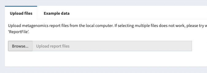
Go to the Pavian website, click on Browse and upload the ERR4998593.report file you have just downloaded.

Once the file is uploaded we can explore the output generated. The column on the left has multiple different options. As we only have one sample and don’t have an alignment to view, only the “Results Overview” and “Sample” tabs are of interest to us.
At the bottom of this column there is also an option to “Generate HTML report”. This is a very good option if you want to share your results with others. We have used that option to generate one here for the ERR4998593 data in order to share our results. If you haven’t been able to generate a Pavian output you can view our exported example here: ERR4998593-pavian-report.html (note this looks a bit different to the website version).
The Results Overview tab shows us how many reads have been classified in our sample(s). From this we can see what proportion of our reads were classified as being bacterial, viral, fungal etc.
On the Sample tab we can see a Sankey diagram which shows us the proportion of our sample that has been classified at each taxa level. If you click on the “Configure Sankey” button you can play with the settings to make the diagram easier to view. Since there are many different species in our Sankey, you might want to try increasing the height of the figure and the number of taxa at each level, to get a broader overview of the species present.
You can also view the Sankey diagram of our example here: sankey-ERR4998593.report.html
Exercise 1: Comparison
Have a look at the Results section of our source paper, where the authors describe some of the genera (subsection 2) and phyla (subsection 3) they documented. Which of our identified taxa match up with the paper’s?
You might find it helpful to import the data from
ERR4998593.reportfile we downloaded into a spreadsheet program (as previously described) to take a more in-depth look at the taxa identified. Remember that you can use filtering to see specific taxonomic levels (e.g. only phyla or only genera). You could also use the search function. Here’s one we made earlier.Solution
The subsection titled “Differences in microbial community structure across soils ecosystems” lists examples genera present in heathland soils (like our sample): Acidipila/Silvibacterium, Bryobacter, Granulicella, Acidothermus, Conexibacter, Mycobacterium, Mucilaginibacter, Bradyrhizobium, and Roseiarcus. Here’s how many of our sequences belong to these genera:
Genus Sequences assigned Bradyrhizobium 154769 Mycobacterium 10863 Granulicella 1344 Conexibacter 2272 Mucilaginibacter 197 Acidothermus 122 Bryobacter 0 Acidipila/Silvibacterium 0 Roseiarcus 0 Note that 298 sequences are assigned to Bryobacteraceae, the family to which the genus Bryobacter belongs. However, all 298 of these sequences are assigned to the genus Paludibaculum, another genus in the Bryobacteraceae family, so we can still confidently say that there are no species belonging to the Bryobacter genus present.
The subsection titled “A manually curated genomic database from tundra soil metagenomes” describes more generally the most represented phyla across the MAGs generated: Acidobacteriota (n = 172), Actinobacteriota (n = 163), Proteobacteria (Alphaproteobacteria, n = 54; Gammaproteobacteria, n = 39), Chloroflexota (n = 84), and Verrucomicrobiota (n = 43). All of these phyla are present in our sample too, albeit in different proportions:
Phylum Sequences assigned Alphaproteobacteria 289043 Actinobacteria 187653 Gammaproteobacteria 18733 Acidobacteria 5500 Verrucomicrobia 778 Chloroflexi 122 The same subsections states that “in general, barren, heathland, and meadow soils were dominated by the same set of MAGs”: Acidobacteriota, Actinobacteria and Proteobacteria. This holds true for our sample, which is taken from a heathland site. Several of the specific genera mentioned (e.g. unclassified genera in class Acidobacteriae, Mycobacterium, Bradyrhizobium, unclassified Xantherobacteraceae and Steroidobacteraceae) are also present.
Exercise 2: Taxonomic level of assignment
What do you think is harder to assign, a species (like E. coli) or a phylum (like Proteobacteria)?
Other software
Krona is a hierarchical data visualization software. Krona allows data to be explored with zooming, multi-layered pie charts and includes support for several bioinformatics tools and raw data formats.
Krona is used in the MG-RAST analysis pipeline which you can read more about at the end of this course.
Key Points
Taxonomy can be assigned by comparing against a database with genome annotations. These are not exhaustive and so many things will remain unannotated depending on the samples you are analysing.
Taxonomic assignment can be done using Kraken2.
Pavian is a web based tool that can be used to visualize the assigned taxa.