QC polished assembly
Overview
Teaching: 30 min
Exercises: 40 minQuestions
Why would we quality control (QC) an assembly?
How can we perform QC on an assembly?
What metrics can we compare between assemblies to understand the quality of an assembly?
Objectives
Understand the terms N50, misassembly and largest contig.
Understand what factors might affect the quality of an assembly.
Use the help documentation to work out an appropriate flag for seqkit
Apply seqkit to assess multiple assemblies
Use metaQUAST to identify the quality of an assembly.
Why QC a metagenome assembly?
We now have a polished assembly. The next thing to do is to perform quality control (QC) checks to make sure we can be confident in our results and conclusions about the taxonomic, metabolic or functional composition of the communities that we are studying. This also allows us to check whether our efforts to improve the assembly with polishing were successful.
The quality of metagenome assemblies is typically lower than it is for single genome assemblies due to the use of long reads.
In this episode we explain what is meant by assembly quality and how to examine and compare the quality of your metagenome assemblies using seqkit stats and MetaQUAST
What do we mean by assembly quality?
There are several variables that affect assembly quality. Let’s go over them in more detail.
Contiguity
A high quality assembly is highly contiguous meaning there are long stretches of the genome that have been successfully pieced together. The opposite of contiguous is fragmented.
Contiguity is strongly correlated with both the technology used and the quality of the original DNA used. “Short read”-only assemblies are often very fragmented as it is much more difficult to assemble the short reads into a contiguous assembly. With long reads it is easier to span bits of a genome that are tricky to reassemble, like repeats. However, some preparation methods, such as bead-beating, result in long-reads which are relatively short.
The extent to which contiguity matters depends on your research question. If you need to identify a large structural difference, high contiguity is important.
Degree of duplication
A duplication is when there is more than one copy of a particular region of the genome in the assembly. If a genome is much bigger than expected then there may have been duplication. Removing duplicated regions from assemblies is difficult but is made easier after the process of binning.
Degree of completeness
The more complete an assembly, the higher quality it is. Sometimes there an regions of the assembly that are unexpectedly missing, meaning the metagenome is incomplete.
Chimeric Contigs
Chimeric contigs are when contigs belonging to different genomes get stuck together as one continuous piece. This is caused during assembly, and can be controlled by the parameters used to generate the assembly. While it is difficult to identify chimeras, it is worth considering the parameters we use for the polishing and assembly steps because inappropriate parameters can result in problems such as these.
Low base quality
Low base quality happens when mutations are present in reads that do not reflect actual biological variation. This happens more in long reads due to a higher error rate. However, this is outweighed by the fact that using long reads for metagenome assemblies results in higher overall quality due to higher contiguity. This is why we ‘polished’ our genome in the last episode by comparing the draft assembly to raw short reads.
Using seqkit to generate summary statistics of an assembly
After finishing the draft assembly we used seqkit stats to see some basic statistics about the assembly. We will be using it again to get summary statistics for all three of the assemblies (unpolished, long read polished and short read polished). We can then use those statistics to examine the polishing process.
We can review the help documentation for seqkit stats.
cd ~/cs_course/analysis/
seqkit stats --help
seqkit stats help documentation
simple statistics of FASTA/Q files

Tips:
  1. For lots of small files (especially on SDD), use big value of '-j' to
     parallelize counting.

Usage:
  seqkit stats [flags]

Aliases:
  stats, stat

Flags:
  -a, --all                  all statistics, including quartiles of seq length, sum_gap, N50
  -b, --basename             only output basename of files
  -E, --fq-encoding string   fastq quality encoding. available values: 'sanger', 'solexa', 'illumina-1.3+', 'illumina-1.5+', 'illumina-1.8+'. (default "sanger")
  -G, --gap-letters string   gap letters (default "- .")
  -h, --help                 help for stats
  -e, --skip-err             skip error, only show warning message
  -i, --stdin-label string   label for replacing default "-" for stdin (default "-")
  -T, --tabular              output in machine-friendly tabular format

Global Flags:
      --alphabet-guess-seq-length int   length of sequence prefix of the first FASTA record based on which seqkit guesses the sequence type (0 for whole seq) (default 10000)
      --id-ncbi                         FASTA head is NCBI-style, e.g. >gi|110645304|ref|NC_002516.2| Pseud...
      --id-regexp string                regular expression for parsing ID (default "^(\\S+)\\s?")
      --infile-list string              file of input files list (one file per line), if given, they are appended to files from cli arguments
  -w, --line-width int                  line width when outputting FASTA format (0 for no wrap) (default 60)
  -o, --out-file string                 out file ("-" for stdout, suffix .gz for gzipped out) (default "-")
      --quiet                           be quiet and do not show extra information
  -t, --seq-type string                 sequence type (dna|rna|protein|unlimit|auto) (for auto, it automatically detect by the first sequence) (default "auto")
  -j, --threads int                     number of CPUs. can also set with environment variable SEQKIT_THREADS) (default 4)
The N50 length
N50 is a metric indicating the distribution of contig lengths in an assembly. The value of N50 indicates that 50% of the total sequence is in contigs that are the that size or larger. For a more thorough introduction to N50, read What’s N50? By The Molecular Ecologist.
It indicates the average size of the contigs the assembly software has produced. A higher N50 length means that more of the assembly is in longer fragments. That means the chunks of sequence produced by the assembler are, on average, larger.
seqkit stats has an option to calculate the N50 length. Use the seqkit stats help documentation to answer the exercise below.
Exercise 1: Flag to get the N50 length
a) Using the help documentation, what flag can we add to get the N50 length for this assembly?
b) What would the new command be if we added this flag?
Bonus exercise: What flag would enable us to save the output table in a tabular (i.e. tsv) format?Solution
a) We can see from the help documentation that the flag
-aor--allwill calculateall statistics, including quartiles of seq length, sum_gap, N50.
b) The new command would beseqkit stats -a assembly/assembly.fastaorseqkit stats --all assembly/assembly.fasta
Bonus: The flag-Tallows us to save it in a tabular output - this makes the table easier to use in other command line programs or programming languages such as R and Python. The command could be eitherseqkit stats -a -T assembly/assembly.fastaor we can combine the two flagsseqkit stats -aT assembly/assembly.fasta
Next, run the command on the original draft assembly (~/cs_course/analysis/assembly/assembly.fasta) to calculate the N50 length and answer the questions below about the output.
Hint: Seqkit stats N50 command
seqkit stats -a assembly/assembly.fasta
Exercise 2: Calculating the N50 length
a) What is the output if we run the new command from the above exercise?
b) What new statistics do we get that we didn’t have with the original command?
c) What is the N50 length of this assembly?Bonus exercise: Looking at the information available online for Seqkit stats, can you work out what the extra statistics other than N50 tell us?
Solution
a)
file                     format  type  num_seqs     sum_len  min_len   avg_len    max_len     Q1      Q2      Q3  sum_gap        N50  Q20(%)  Q30(%)  GC(%)
assembly/assembly.fasta  FASTA   DNA        154  15,042,667    3,164  97,679.7  6,068,626  7,305  13,291  34,356        0  2,976,488       0       0  52.39
b) Comparing the header line from this command to the original command we can see we’ve now got statistics for Q1, Q2, Q3, sum_gap, N50, Q20(%) and Q30(%)
c) The N50 length for this assembly is 2,976,503 bp. This tells us that 50% of the assembly is in fragments that are almost 3m bases long or longer!Bonus:
Q1,Q2andQ3are the quartile ranges of sequence length.sum_gapis the total number of ambiguous bases (N’s) in the sequence.Q20(%) is the percentage of bases with a PHRED score over 20 and similarlyQ30(%) is the percentage of bases with a PHRED score over 30. GC(%) is the guanine-cytosine content of the sequence.
Generating statistics for all three assemblies
Instead of passing just one FASTA file to seqkit stats we can use all three FASTA files at once.
First we need to navigate into the analysis directory.
cd ~/cs_course/analysis/
Within the analysis directory, these three files are:
- Draft assembly generated by Flye in
assembly/assembly.fasta - Long-read polished assembly generated by Medaka in
medaka/consensus.fasta - Short-read polished assembly generated by Pilon in
pilon/pilon.fasta
This makes our command:
seqkit stats -a assembly/assembly.fasta medaka/consensus.fasta pilon/pilon.fasta
| file | format | type | num_seqs | sum_len | min_len | avg_len | max_len | Q1 | Q2 | Q3 | sum_gap | N50 | Q20(%) | Q30(%) | GC(%) |
|---|---|---|---|---|---|---|---|---|---|---|---|---|---|---|---|
| assembly/assembly.fasta | FASTA | DNA | 154 | 15042667 | 3164 | 97679.7 | 6068626 | 7305.0 | 13291.0 | 34356.0 | 0 | 2976488 | 0.00 | 0.00 | 52.39 |
| medaka/consensus.fasta | FASTA | DNA | 154 | 15062138 | 3142 | 97806.1 | 6074421 | 7166.0 | 13265.5 | 34010.0 | 0 | 2991856 | 0.00 | 0.00 | 52.30 |
| pilon/pilon.fasta | FASTA | DNA | 154 | 15070837 | 3144 | 97862.6 | 6074532 | 7175.0 | 13279.5 | 34010.0 | 0 | 2992063 | 0.00 | 0.00 | 52.27 |
Exercise 3: Comparing the Assemblies
Using the seqkit output for all three assemblies, compare the statistics for each of the three assemblies. What has changed across the two rounds of polishing? (From assembly>medaka>pilon)
Solution
Between the original assembly and the medaka polished assembly:
- Total length, maximum length and average length have all increased as has the N50, the minimum length and GC content have decreased as has the quartile range of lengths.
Between the medaka polished assembly and the pilon polished assembly:
- The total length, average length, maximum length, Q1, Q2, minimum length and N50 have all increased. The GC% and Q3 have decreased.
We can compare these basic assembly statistics in this way. However, these may not tell the full story as there will also have been changes to the overall sequence (e.g. correcting individual base errors).
Using metaQUAST to further assess assembly quality
We will use MetaQUAST to further evaluate our metagenomic assemblies. MetaQUAST is based on the QUAST genome quality tool but accounts for high species divesity and misassemblies.
MetaQUAST assesses the quality of assemblies using alignments to close references. This means we need to determine which references are appropriate for our data. MetaQUAST can automatically select reference genomes to align the assembly to, but it does not always pick the most appropriate references. As we know what organisms make up our metagenome we will be supplying a file containing the references we want to use instead. If you use MetaQUAST on your own data you could use the default references MetaQUAST selects or provide your own if you have an idea what organisms could be in your dataset.
So far we’ve been able to do a lot of work with files that already exist, but now we need to write our own file using the text editor Nano.
Text editors
Text editors, like nano, “notepad” on Windows or “TextEdit” on Mac are used to edit any plain text files. Plain text files are those that contain only characters, not images or formatting.
We are using nano because it is one of the least complex Unix text editors. However, many programmers use Emacs or Vim (both of which require more time to learn), or a graphical editor such as Gedit.
No matter what editor you use, you will need to know where it searches for and saves files. If you start it from the shell, it will (probably) use your current working directory as its default location.
Writing files
First, we create a directory for the metaQUAST output in the analysis directory.
cd ~/cs_course/analysis/
mkdir metaquast
cd metaquast
To open nano we type the command nano followed by the name of the text file we want to generate.
nano reference_genomes.txt
You should see something like this:
The text at the bottom of the screen shows the keyboard shortcuts for performing various tasks in nano. We will talk more about how to interpret this information soon.
When you press enter your terminal should change. You should see a white bar at the top with GNU nano 4.8 and some suggested commands at the bottom of the page.
There should also be a white box which indicates where your cursor is.
Paste the following list of organism names into this file.
Bacillus subtilis
Cryptococcus neoformans
Enterococcus faecalis
Escherichia coli str. K-12 substr. MG1655
Lactobacillus fermentum
Listeria monocytogenes EGD-e
Pseudomonas aeruginosa
Saccharomyces cerevisiae
Salmonella enterica subsp. enterica serovar Typhimurium str. LT2
Staphylococcus aureus
Once we’re happy with our text, we can press Ctrl-O (press the Ctrl or Control key and, while holding it down, press the O key) to write our data to disk. You will the be prompted with File Name to Write: reference_genomes.txt as we named the file when we first used the command we don’t need to change this name and can press Enter to save the file. Once our file is saved, we can use Ctrl-X to quit the nano editor and
return to the shell.
Control, Ctrl, or ^ Key
The Control key is also called the “Ctrl” key. There are various ways in which using the Control key may be described. For example, you may see an instruction to press the Ctrl key and, while holding it down, press the X key, described as any of:
Control-XControl+XCtrl-XCtrl+X^XC-xIn
nano, along the bottom of the screen you’ll see^G Get Help ^O WriteOut. This means that you can use Ctrl-G to get help and Ctrl-O to save your file.If you are using a Mac, you might be more familiar with the
Commandkey, which is labelled with a ⌘ . But you will often use the theCtrlkey when working in a Terminal.
Copying and pasting in Git bash
Most people will want to use Ctrl+C and Ctrl+V to copy and paste. However in GitBash these shortcuts have other functions. Ctrl+C interrupts the currently running command and Ctrl+V tells the terminal to treat every keystroke as a literal character, so will add shortcuts like Ctrl+C as characters. Instead you can copy and paste in two ways:
- Keyboard: Use Shift and the left/right arrows to select text and press Enter to copy. You can paste the text by pressing Insert.
- Mouse: Left click and drag to highlight text, then right click to copy. Move the cursor to where you want to paste and right click to paste.
You should then be able to see this file when you ls and view it using less.
ls
reference_genomes.txt
Once we have our list of reference genomes we can run MetaQUAST on the original assembly and the two polished assemblies.
First we should look at the help documentation to work out which commands are right for us.
metaquast.py -h
MetaQUAST help documentation
MetaQUAST: Quality Assessment Tool for Metagenome Assemblies
Version: 5.2.0

Usage: python metaquast.py [options] <files_with_contigs>

Options:
-o  --output-dir  <dirname>       Directory to store all result files [default: quast_results/results_<datetime>]
-r   <filename,filename,...>      Comma-separated list of reference genomes or directory with reference genomes
--references-list <filename>      Text file with list of reference genome names for downloading from NCBI
-g  --features [type:]<filename>  File with genomic feature coordinates in the references (GFF, BED, NCBI or TXT)
                                  Optional 'type' can be specified for extracting only a specific feature type from GFF
-m  --min-contig  <int>           Lower threshold for contig length [default: 500]
-t  --threads     <int>           Maximum number of threads [default: 25% of CPUs]

Advanced options:
-s  --split-scaffolds                 Split assemblies by continuous fragments of N's and add such "contigs" to the comparison
-l  --labels "label, label, ..."      Names of assemblies to use in reports, comma-separated. If contain spaces, use quotes
-L                                    Take assembly names from their parent directory names
-e  --eukaryote                       Genome is eukaryotic (primarily affects gene prediction)
    --fungus                          Genome is fungal (primarily affects gene prediction)
    --large                           Use optimal parameters for evaluation of large genomes
                                      In particular, imposes '-e -m 3000 -i 500 -x 7000' (can be overridden manually)
-k  --k-mer-stats                     Compute k-mer-based quality metrics (recommended for large genomes)
                                      This may significantly increase memory and time consumption on large genomes
    --k-mer-size                      Size of k used in --k-mer-stats [default: 101]
    --circos                          Draw Circos plot
-f  --gene-finding                    Predict genes using MetaGeneMark
    --glimmer                         Use GlimmerHMM for gene prediction (instead of the default finder, see above)
    --gene-thresholds <int,int,...>   Comma-separated list of threshold lengths of genes to search with Gene Finding module
                                      [default: 0,300,1500,3000]
    --rna-finding                     Predict ribosomal RNA genes using Barrnap
-b  --conserved-genes-finding         Count conserved orthologs using BUSCO (only on Linux)
    --operons  <filename>             File with operon coordinates in the reference (GFF, BED, NCBI or TXT)
    --max-ref-number <int>            Maximum number of references (per each assembly) to download after looking in SILVA database.
                                      Set 0 for not looking in SILVA at all [default: 50]
    --blast-db <filename>             Custom BLAST database (.nsq file). By default, MetaQUAST searches references in SILVA database
    --use-input-ref-order             Use provided order of references in MetaQUAST summary plots (default order: by the best average value)
    --contig-thresholds <int,int,...> Comma-separated list of contig length thresholds [default: 0,1000,5000,10000,25000,50000]
    --x-for-Nx <int>                  Value of 'x' for Nx, Lx, etc metrics reported in addition to N50, L50, etc (0, 100) [default: 90]
    --reuse-combined-alignments       Reuse the alignments from the combined_reference stage on runs_per_reference stages.
-u  --use-all-alignments              Compute genome fraction, # genes, # operons in QUAST v1.* style.
                                      By default, QUAST filters Minimap's alignments to keep only best ones
-i  --min-alignment <int>             The minimum alignment length [default: 65]
    --min-identity <float>            The minimum alignment identity (80.0, 100.0) [default: 90.0]
-a  --ambiguity-usage <none|one|all>  Use none, one, or all alignments of a contig when all of them
                                      are almost equally good (see --ambiguity-score) [default: one]
    --ambiguity-score <float>         Score S for defining equally good alignments of a single contig. All alignments are sorted
                                      by decreasing LEN * IDY% value. All alignments with LEN * IDY% < S * best(LEN * IDY%) are
                                      discarded. S should be between 0.8 and 1.0 [default: 0.99]
    --unique-mapping                  Disable --ambiguity-usage=all for the combined reference run,
                                      i.e. use user-specified or default ('one') value of --ambiguity-usage
    --strict-NA                       Break contigs in any misassembly event when compute NAx and NGAx.
                                      By default, QUAST breaks contigs only by extensive misassemblies (not local ones)
-x  --extensive-mis-size  <int>       Lower threshold for extensive misassembly size. All relocations with inconsistency
                                      less than extensive-mis-size are counted as local misassemblies [default: 1000]
    --local-mis-size  <int>           Lower threshold on local misassembly size. Local misassemblies with inconsistency
                                      less than local-mis-size are counted as (long) indels [default: 200]
    --scaffold-gap-max-size  <int>    Max allowed scaffold gap length difference. All relocations with inconsistency
                                      less than scaffold-gap-size are counted as scaffold gap misassemblies [default: 10000]
    --unaligned-part-size  <int>      Lower threshold for detecting partially unaligned contigs. Such contig should have
                                      at least one unaligned fragment >= the threshold [default: 500]
    --skip-unaligned-mis-contigs      Do not distinguish contigs with >= 50% unaligned bases as a separate group
                                      By default, QUAST does not count misassemblies in them
    --fragmented                      Reference genome may be fragmented into small pieces (e.g. scaffolded reference)
    --fragmented-max-indent  <int>    Mark translocation as fake if both alignments are located no further than N bases
                                      from the ends of the reference fragments [default: 200]
                                      Requires --fragmented option
    --upper-bound-assembly            Simulate upper bound assembly based on the reference genome and reads
    --upper-bound-min-con  <int>      Minimal number of 'connecting reads' needed for joining upper bound contigs into a scaffold
                                      [default: 2 for mate-pairs and 1 for long reads]
    --est-insert-size  <int>          Use provided insert size in upper bound assembly simulation [default: auto detect from reads or 255]
    --report-all-metrics              Keep all quality metrics in the main report even if their values are '-' for all assemblies or
                                      if they are not applicable (e.g., reference-based metrics in the no-reference mode)
    --plots-format  <str>             Save plots in specified format [default: pdf].
                                      Supported formats: emf, eps, pdf, png, ps, raw, rgba, svg, svgz
    --memory-efficient                Run everything using one thread, separately per each assembly.
                                      This may significantly reduce memory consumption on large genomes
    --space-efficient                 Create only reports and plots files. Aux files including .stdout, .stderr, .coords will not be created.
                                      This may significantly reduce space consumption on large genomes. Icarus viewers also will not be built
-1  --pe1     <filename>              File with forward paired-end reads (in FASTQ format, may be gzipped)
-2  --pe2     <filename>              File with reverse paired-end reads (in FASTQ format, may be gzipped)
    --pe12    <filename>              File with interlaced forward and reverse paired-end reads. (in FASTQ format, may be gzipped)
    --mp1     <filename>              File with forward mate-pair reads (in FASTQ format, may be gzipped)
    --mp2     <filename>              File with reverse mate-pair reads (in FASTQ format, may be gzipped)
    --mp12    <filename>              File with interlaced forward and reverse mate-pair reads (in FASTQ format, may be gzipped)
    --single  <filename>              File with unpaired short reads (in FASTQ format, may be gzipped)
    --pacbio     <filename>           File with PacBio reads (in FASTQ format, may be gzipped)
    --nanopore   <filename>           File with Oxford Nanopore reads (in FASTQ format, may be gzipped)
    --ref-sam <filename>              SAM alignment file obtained by aligning reads to reference genome file
    --ref-bam <filename>              BAM alignment file obtained by aligning reads to reference genome file
    --sam     <filename,filename,...> Comma-separated list of SAM alignment files obtained by aligning reads to assemblies
                                      (use the same order as for files with contigs)
    --bam     <filename,filename,...> Comma-separated list of BAM alignment files obtained by aligning reads to assemblies
                                      (use the same order as for files with contigs)
                                      Reads (or SAM/BAM file) are used for structural variation detection and
                                      coverage histogram building in Icarus
    --sv-bedpe  <filename>            File with structural variations (in BEDPE format)

Speedup options:
    --no-check                        Do not check and correct input fasta files. Use at your own risk (see manual)
    --no-plots                        Do not draw plots
    --no-html                         Do not build html reports and Icarus viewers
    --no-icarus                       Do not build Icarus viewers
    --no-snps                         Do not report SNPs (may significantly reduce memory consumption on large genomes)
    --no-gc                           Do not compute GC% and GC-distribution
    --no-sv                           Do not run structural variation detection (make sense only if reads are specified)
    --no-read-stats                   Do not align reads to assemblies
                                      Reads will be aligned to reference and used for coverage analysis,
                                      upper bound assembly simulation, and structural variation detection.
                                      Use this option if you do not need read statistics for assemblies.
    --fast                            A combination of all speedup options except --no-check

Other:
    --silent                          Do not print detailed information about each step to stdout (log file is not affected)
    --test                            Run MetaQUAST on the data from the test_data folder, output to quast_test_output
    --test-no-ref                     Run MetaQUAST without references on the data from the test_data folder, output to quast_test_output.
                                      MetaQUAST will download SILVA 16S rRNA database (~170 Mb) for searching reference genomes
                                      Internet connection is required
-h  --help                            Print full usage message
-v  --version                         Print version

Online QUAST manual is available at http://quast.sf.net/manual
From this we can see we need --references-list to supply our list of reference organisms (this is the file we just made called reference_genomes.txt), followed by our three assemblies separated by a space.
metaquast.py --references-list reference_genomes.txt ../assembly/assembly.fasta ../medaka/consensus.fasta ../pilon/pilon.fasta
This should take around 5 minutes so we will be leaving it running in the foreground.
Once starting the command you should see something like this and metaQUAST will start downloading the reference species we specified in our files.
Version: 5.2.0

System information:
  OS: Linux-3.10.0
  Python version: 3.10.5
  CPUs number: 4

Started: 2022-09-26 17:26:14

Logging to analysis/metaquast/quast_results/results_2022_09_26_17_26_13/metaquast.log
NOTICE: Maximum number of threads is set to 10 (use --threads option to set it manually)

Contigs:
  Pre-processing...
  1  ../assembly/assembly.fasta ==> assembly
  2  ../medaka/consensus.fasta ==> consensus
  3  ../pilon/pilon.fasta ==> pilon

List of references was provided, starting to download reference genomes from NCBI...

2022-09-26 17:26:31

2022-09-26 17:26:31
Trying to download found references from NCBI. Totally 10 organisms to try.
  Bacillus_subtilis                                                | successfully downloaded (total 1, 9 more to go)
  Cryptococcus_neoformans                                          | successfully downloaded (total 2, 8 more to go)
  Enterococcus_faecalis                                            | successfully downloaded (total 3, 7 more to go)
  Escherichia_coli_str._K-12_substr._MG1655                        | successfully downloaded (total 4, 6 more to go)
  Lactobacillus_fermentum                                          | successfully downloaded (total 5, 5 more to go)
  Listeria_monocytogenes_EGD-e                                     | successfully downloaded (total 6, 4 more to go)
  Pseudomonas_aeruginosa                                           | successfully downloaded (total 7, 3 more to go)
  Saccharomyces_cerevisiae                                         | successfully downloaded (total 8, 2 more to go)
  Salmonella_enterica_subsp._enterica_serovar_Typhimurium_str._LT2 | successfully downloaded (total 9, 1 more to go)
  Staphylococcus_aureus                                            | successfully downloaded (total 10, 0 more to go)
Once MetaQUAST has finished you should see an output like:
MetaQUAST finished.
  Log is saved to analysis/metaquast/quast_results/results_2022_09_26_17_26_13/metaquast.log

Finished: 2022-09-26 17:31:00
Elapsed time: 0:04:45.735581
Total NOTICEs: 13; WARNINGs: 1; non-fatal ERRORs: 0

Thank you for using QUAST!
We can now navigate into the quast_results directory MetaQUAST generated. Within this directory there will be a folder for each time MetaQUAST has been run in this directory. We can navigate then navigate into the results file generated which will be in the format results_YYYY_MM_DD_HH_MM_SS. (There is also a symbolic link called latest in this directory that is a shortcut to the newest MetaQUAST run).
cd quast_results/results_YYYY_MM_DD_HH_MM_SS/
ls
combined_reference icarus.html icarus_viewers metaquast.log not_aligned quast_downloaded_references report.html runs_per_reference summary
Once in this directory, we can see that MetaQUAST has generated multiple different files.
If you want to explore all the files you can download this whole directory using scp, with -r flag to download all directories and what they contain. This will require ~500MB of space.
However, most of this information is in the report.html file so we can download only that one instead.
As this is a HTML file we will first need to download it to our local computer in order to open it.
scp -i login-key-instanceNNN.pem csuser@instanceNNN.cloud-span.aws.york.ac.uk:~/cs_course/analysis/metaquast/quast_results/results_YYYY_MM_DD_HH_MM_SS/report.html .
Make sure you replace both the NNN with your particular number and also the directory name of the results file.
The results.html file relies on some of the other files generated by MetaQUAST so with only the one file you won’t have full functionality but we can still view the information we want.
If you haven’t managed to download the file you can view our example report.html
You should take a few minutes to explore the file before answering the following exercise.
Understanding metaQUAST output
The output is organised into several sections, with a column for each assembly. The worst scoring column is shown in red, the best in blue.
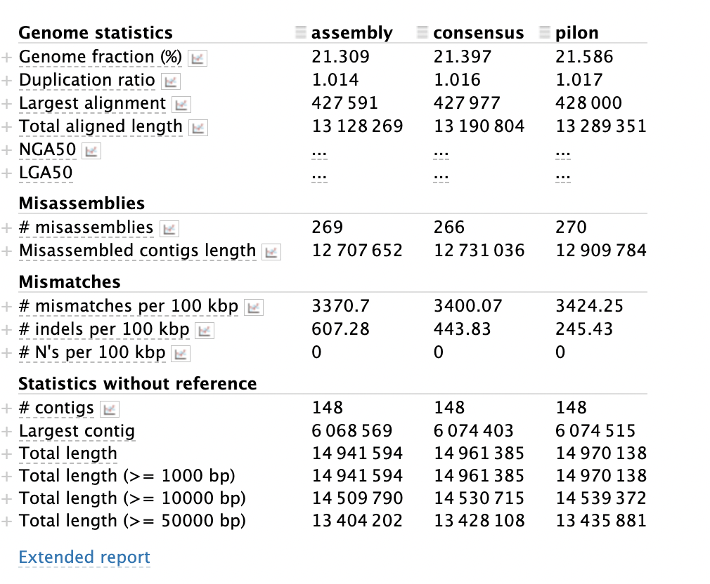
Genome statistics
This section determines the quality of the assembly based on the size of the total assembly. The duplication ratio is the amount of the total assembly that is represented more than once. The more fragmented the assembly, the higher this value will be. See What makes an assembly bad section above to see further details.
Misassemblies
Missassemblies are when pieces in an assembly are overlapped in the incorrect way. In the metaQUAST manual, they define missassemblies in the four following ways (taken from the manual):
misassemblies is the number of positions in the contigs (breakpoints) that satisfy one of the following criteria.
- the left flanking sequence aligns over 1 kbp away from the right flanking sequence on the reference;
- flanking sequences overlap on more than 1 kbp;
- flanking sequences align to different strands or different chromosomes;
- flanking sequences align on different reference genomes (MetaQUAST only)
These can be caused by errors in the assembly, or they can be caused my structural variation in the sample, such as inversions, relocations and translocation.
Mismatches
This is where there are incorrect bases in the contigs making up the assembly. The summary gives you the total number of mismatches per 100kbp of sequence and short insertions and deletions (indels) per 100kbp.
Statistics without reference
The statistics without a reference are based on the full assembly rather than comparing the assembly to the species that you have asked it to compare to. The largest contig is an indicator of how good the overall assembly is. If the largest contig is small, it means that the rest of the assembly is of a poor quality.
There is a detailed description of each of the outputs in the metaQUAST manual which you can use to understand the output more fully.
Comparing assemblies using MetaQUAST
Using the above image how has the iterative polishing from assembly > consensus > pilon improved the assembly?
Answer
In the pilon assembly we have improved the assembly is some ways, but worsened the assembly in others. In the final assembly we have a more complete assembly (see genome fraction). We have also increased the total length of the assembly (see total aligned length and Statistics without reference section). The downside of increasing the length is that we may have introduced some missassemblies and duplicated bits of the assembly (see Misassemblies section). This complexity in different statistics showing the assembly is improved and others worse, illustrates the difficulty in assessing the quality of an assembly.
Key Points
The N50 is the contig length of the 50th percentile, meaning that 50% of the contigs are at least this length in the assembly
A misassembly is when a portion of the assembly is incorrectly put back together
The largest contig is the longest contiguous piece in the assembly
Seqkit can generate summary statistics that will tell us the N50, largest contig and the number of gaps
metaQUAST can generate additional information in a report which can be used to identify misassemblies