Variant Calling Workflow
Overview
Teaching: 35 min
Exercises: 25 minQuestions
How do I find sequence variants between my sample and a reference genome?
Objectives
Understand the steps involved in variant calling.
Describe the types of data formats encountered during variant calling.
Use command line tools to perform variant calling.
We mentioned before that we are working with files from a long-term evolution study of an E. coli population (designated Ara-3). Now that we have looked at our data to make sure that it is high quality, and removed low-quality base calls, we can perform variant calling to see how the population changed over time. We care how this population changed relative to the original population, E. coli strain REL606. Therefore, we will align each of our samples to the E. coli REL606 reference genome, and see what differences exist in our reads versus the genome.
Alignment to a reference genome
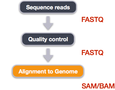
We perform read alignment or mapping to determine where in the genome our reads originated from. There are a number of tools to choose from and, while there is no gold standard, there are some tools that are better suited for particular NGS analyses. We will be using the Burrows Wheeler Aligner (BWA), which is a software package for mapping low-divergent sequences against a large reference genome.
The alignment process consists of two steps:
- Indexing the reference genome
- Aligning the reads to the reference genome
Setting up
First we download the reference genome for E. coli REL606. Although we could copy or move the file with cp or mv, most genomics workflows begin with a download step, so we will practice that here.
$ cd ~/cs_course
$ curl -L -o data/ecoli_rel606.fasta.gz ftp://ftp.ncbi.nlm.nih.gov/genomes/all/GCA/000/017/985/GCA_000017985.1_ASM1798v1/GCA_000017985.1_ASM1798v1_genomic.fna.gz
The -L flag stands for location. If the server reports that the requested page has moved then curl will redo the request on the new page. The -o flag means the output goes to a file rather than the terminal.
The file ecoli_rel606.fasta.gz has been dowloaded to the data folder since we specified data/ecoli_rel606.fasta.gz in the curl command. This file needs to be decompressed (unzipped) with:
$ gunzip data/ecoli_rel606.fasta.gz
Exercise
We saved this file as
data/ecoli_rel606.fasta.gzand then decompressed it. What is the real name of the genome?Hint: the name of the genome is often recorded at the top of the file.
Solution
$ head data/ecoli_rel606.fastaThe name of the sequence follows the
>character. The name isCP000819.1 Escherichia coli B str. REL606, complete genome. Keep this chromosome name (CP000819.1) in mind, as we will use it later in the lesson.
We will also download a set of trimmed FASTQ files to work with. These are small subsets of our real trimmed data, and will enable us to run our variant calling workflow quite quickly.
$ curl -L -o sub.tar.gz https://ndownloader.figshare.com/files/14418248
The sub.tar.gz file also needs to be decompressed.
$ tar xvf sub.tar.gz
You now have a folder, sub containing six .fastq files.
Let’s put this folder inside of data folder using mv. Since the name sub is not very informative, we can rename it to trimmed_fastq_small at the same time.
$ mv sub/ ~/cs_course/data/trimmed_fastq_small
Index the reference genome
Our first step is to index the reference genome for use by BWA. Indexing allows the aligner to quickly find potential alignment sites for query sequences in a genome, which saves time during alignment. Indexing the reference only has to be run once. The only reason you would want to create a new index is if you are working with a different reference genome or you are using a different tool for alignment.
$ bwa index data/ecoli_rel606.fasta
While the index is created, you will see output that looks something like this:
[bwa_index] Pack FASTA... 0.04 sec
[bwa_index] Construct BWT for the packed sequence...
[bwa_index] 1.05 seconds elapse.
[bwa_index] Update BWT... 0.03 sec
[bwa_index] Pack forward-only FASTA... 0.02 sec
[bwa_index] Construct SA from BWT and Occ... 0.57 sec
[main] Version: 0.7.17-r1188
[main] CMD: bwa index data/ecoli_rel606.fasta
[main] Real time: 1.765 sec; CPU: 1.715 sec
Align reads to reference genome
The alignment process consists of choosing an appropriate reference genome to map our reads against and then deciding on an aligner. We will use the BWA-MEM algorithm, which is the latest and is generally recommended for high-quality queries as it is faster and more accurate.
An example of what a bwa command looks like is below. This command will not run, as we do not have the files ref_genome.fa, input_file_R1.fastq, or input_file_R2.fastq.
$ bwa mem ref_genome.fasta input_file_R1.fastq input_file_R2.fastq > output.sam
Have a look at the bwa options page. While we are running bwa with the default parameters here, your use case might require a change of parameters. NOTE: Always read the manual page for any tool before using and make sure the options you use are appropriate for your data.
We’re going to start by aligning the reads from just one of the
samples in our dataset (SRR2584866).
$ bwa mem data/ecoli_rel606.fasta data/trimmed_fastq_small/SRR2584866_1.trim.sub.fastq data/trimmed_fastq_small/SRR2584866_2.trim.sub.fastq > results/SRR2584866.aligned.sam
You will see output that starts like this:
[M::bwa_idx_load_from_disk] read 0 ALT contigs
[M::process] read 77446 sequences (10000033 bp)...
[M::process] read 77296 sequences (10000182 bp)...
[M::mem_pestat] # candidate unique pairs for (FF, FR, RF, RR): (48, 36728, 21, 61)
[M::mem_pestat] analysing insert size distribution for orientation FF...
[M::mem_pestat] (25, 50, 75) percentile: (420, 660, 1774)
[M::mem_pestat] low and high boundaries for computing mean and std.dev: (1, 4482)
[M::mem_pestat] mean and std.dev: (784.68, 700.87)
[M::mem_pestat] low and high boundaries for proper pairs: (1, 5836)
[M::mem_pestat] analysing insert size distribution for orientation FR...
BWA Alignment options
BWA consists of three algorithms: BWA-backtrack, BWA-SW and BWA-MEM. The first algorithm is designed for Illumina sequence reads up to 100bp, while the other two are for sequences ranging from 70bp to 1Mbp. BWA-MEM and BWA-SW share similar features such as long-read support and split alignment, but BWA-MEM, which is the latest, is generally recommended for high-quality queries as it is faster and more accurate.
SAM/BAM format
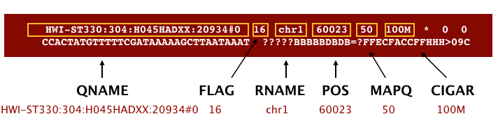
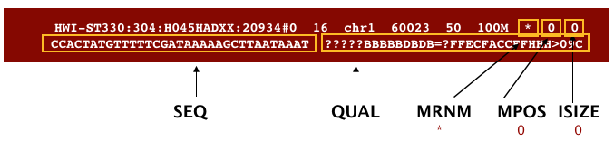
The SAM file, is a tab-delimited text file that contains information for each individual read and its alignment to the genome. While we do not have time to go into detail about the features of the SAM format, the paper by Heng Li et al. provides a lot more detail on the specification.
The compressed binary version of SAM is called a BAM file. We use this version to reduce size and to allow for indexing, which enables efficient random access of the data contained within the file.
The file begins with a header, which is optional. The header is used to describe the source of data, reference sequence, method of alignment, etc., this will change depending on the aligner being used. Following the header is the alignment section. Each line that follows corresponds to alignment information for a single read. Each alignment line has 11 mandatory fields for essential mapping information and a variable number of other fields for aligner specific information. An example entry from a SAM file is displayed below with the different fields highlighted.
We will convert the SAM file to BAM format using the samtools program with the view command. There are a couple of options/flags we need to include:
-Stells samtools that the input is in SAM format-btells samtools that the output should be in BAM format
$ cd results
$ samtools view -S -b SRR2584866.aligned.sam > SRR2584866.aligned.bam
Sort BAM file by coordinates
Next we sort the BAM file using the sort command from samtools. The default setting for this command is to sort the alignments by coordinates i.e. where they lie on the chromosome.
-otells the command to write the sorted output to a file calledSRR2584866.aligned.sorted.bam
$ samtools sort -o SRR2584866.aligned.sorted.bam SRR2584866.aligned.bam
Our files are pretty small, so we won’t see this output. If you run the workflow with larger files, you will see something like this:
[bam_sort_core] merging from 2 files...
SAM/BAM files can be sorted in multiple ways, e.g. by location of alignment on the chromosome, by read name, etc. It is important to be aware that different alignment tools will output differently sorted SAM/BAM, and different downstream tools require differently sorted alignment files as input.
Index the sorted BAM file
We will now index our sorted BAM file. This will generate a bam.bai file which we will need later on.
When we indexed the reference genome we used bwa because we were working with a FASTA file. This time we are working with a BAM file so we’ll use samtools instead, but the general principle is the same.
samtools index SRR2584866.aligned.sorted.bam
BAM statistics
You can use samtools to learn more about the sorted BAM file as well.
samtools flagstat SRR2584866.aligned.sorted.bam
This will give you the following statistics about your file:
351169 + 0 in total (QC-passed reads + QC-failed reads)
0 + 0 secondary
1169 + 0 supplementary
0 + 0 duplicates
351103 + 0 mapped (99.98% : N/A)
350000 + 0 paired in sequencing
175000 + 0 read1
175000 + 0 read2
346688 + 0 properly paired (99.05% : N/A)
349876 + 0 with itself and mate mapped
58 + 0 singletons (0.02% : N/A)
0 + 0 with mate mapped to a different chr
0 + 0 with mate mapped to a different chr (mapQ>=5)
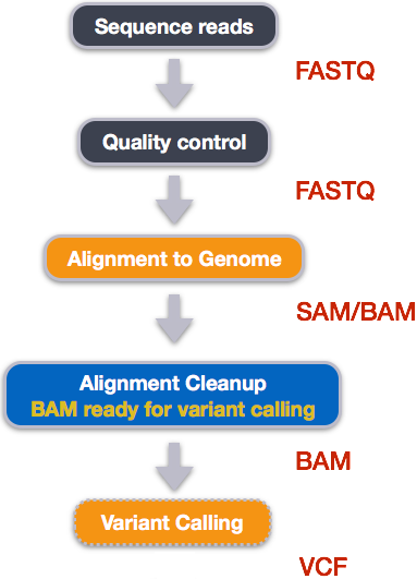
Variant calling
A variant call is a conclusion that there is a nucleotide difference vs. some reference at a given position in an individual genome
or transcriptome, often referred to as a Single Nucleotide Polymorphism (SNP). The call is usually accompanied by an estimate of
variant frequency and some measure of confidence. Similar to other steps in this workflow, there are a number of tools available for
variant calling. In this workshop we will be using bcftools, but there are a few things we need to do before actually calling the
variants.
Step 1: Calculate the read coverage of positions in the genome
Do the first pass on variant calling by counting read coverage with bcftools. We will
use the command mpileup, which is one method of summarising the coverage of mapped reads at single base pair resolution. There are other tools which do the same job, such as GATK and freebayes.
-O bbcftools to generate the output file in BCF formatoindicates that the output should be calledSRR2584866_raw.bcfftells bcftools to find the reference genome at the path../data/ecoli_rel606.fasta SRR2584866.aligned.sorted.bam
$ bcftools mpileup -O b -o SRR2584866_raw.bcf \
-f ../data/ecoli_rel606.fasta SRR2584866.aligned.sorted.bam
[mpileup] 1 samples in 1 input files
[mpileup] maximum number of reads per input file set to -d 250
We have now generated a file with coverage information for every base.
Step 2: Detect the single nucleotide polymorphisms (SNPs)
Now we can look through our aligned reads and identify SNPs using bcftools call. Once again there are some parameters we need to specify:
--ploidyindicates the ploidy of the genome being analysed - in our case, E. coli is haploidy so this is1-mtells bcftools that multiallelic and rare-variant calls are allowed (this allows more than one variant allele at any given position)-vtells bcftools to output variant sites only-otells bcftools to write the output to a file calledSRR2584866_variants.vcf
$ bcftools call --ploidy 1 -m -v -o SRR2584866_variants.vcf SRR2584866_raw.bcf
Step 3: Filter and report the SNP variants in variant calling format (VCF)
Now we will filter the SNPs to exclude those which are not robustly supported changes. For this we will use a script called vcfutils.pl, which has a function called varFilter. Our output will be in VCF format.
This is not the only way to filter SNPs. However, it is useful because it already has a set of default filters which makes our lives a bit easier! Some of the filters it implements include:
- minimum root mean square (RMS) of mapping quality i.e. the minimum acceptable probability that a read is incorrectly aligned (default = 10)
- minimum read depth i.e. the minimum number of reads covering that locus (default = 2)
- maximum read depth (default = 10000000)
- minimum number of alternate reads supporting the SNP (default = 2)
- minimum distance from a gap (a region not covered by any mapped reads) (default = 3)
To run the script with default parameters:
$ vcfutils.pl varFilter SRR2584866_variants.vcf > SRR2584866_final_variants.vcf
Useful info
Today we will use the default filters but it may be useful to try applying different parameters in your own time to see what difference they make to the final SNP report. You can find a list of the filters used on line 223 of this script
To change the value of a parameter from the default, add it to the command using the appropriate flag. For example:
$ vcfutils.pl varFilter -d 5 SRR2584866_variants.vcf > SRR2584866_final_variants.vcfsets the minimum read depth (-d) to 5.
Explore the VCF format:
$ less -S SRR2584866_final_variants.vcf
You will see the header (which describes the format), the time and date the file was created, the version of bcftools that was used, the command line parameters used, and some additional information:
##fileformat=VCFv4.2
##FILTER=<ID=PASS,Description="All filters passed">
##bcftoolsVersion=1.8+htslib-1.8
##bcftoolsCommand=mpileup -O b -o SRR2584866_raw.bcf -f data/ecoli_rel606.fasta SRR2584866.aligned.sorted.bam
##reference=file://data/ecoli_rel606.fasta
##contig=<ID=CP000819.1,length=4629812>
##ALT=<ID=*,Description="Represents allele(s) other than observed.">
##INFO=<ID=INDEL,Number=0,Type=Flag,Description="Indicates that the variant is an INDEL.">
##INFO=<ID=IDV,Number=1,Type=Integer,Description="Maximum number of reads supporting an indel">
##INFO=<ID=IMF,Number=1,Type=Float,Description="Maximum fraction of reads supporting an indel">
##INFO=<ID=DP,Number=1,Type=Integer,Description="Raw read depth">
##INFO=<ID=VDB,Number=1,Type=Float,Description="Variant Distance Bias for filtering splice-site artefacts in RNA-seq data (bigger is better)",Version=
##INFO=<ID=RPB,Number=1,Type=Float,Description="Mann-Whitney U test of Read Position Bias (bigger is better)">
##INFO=<ID=MQB,Number=1,Type=Float,Description="Mann-Whitney U test of Mapping Quality Bias (bigger is better)">
##INFO=<ID=BQB,Number=1,Type=Float,Description="Mann-Whitney U test of Base Quality Bias (bigger is better)">
##INFO=<ID=MQSB,Number=1,Type=Float,Description="Mann-Whitney U test of Mapping Quality vs Strand Bias (bigger is better)">
##INFO=<ID=SGB,Number=1,Type=Float,Description="Segregation based metric.">
##INFO=<ID=MQ0F,Number=1,Type=Float,Description="Fraction of MQ0 reads (smaller is better)">
##FORMAT=<ID=PL,Number=G,Type=Integer,Description="List of Phred-scaled genotype likelihoods">
##FORMAT=<ID=GT,Number=1,Type=String,Description="Genotype">
##INFO=<ID=ICB,Number=1,Type=Float,Description="Inbreeding Coefficient Binomial test (bigger is better)">
##INFO=<ID=HOB,Number=1,Type=Float,Description="Bias in the number of HOMs number (smaller is better)">
##INFO=<ID=AC,Number=A,Type=Integer,Description="Allele count in genotypes for each ALT allele, in the same order as listed">
##INFO=<ID=AN,Number=1,Type=Integer,Description="Total number of alleles in called genotypes">
##INFO=<ID=DP4,Number=4,Type=Integer,Description="Number of high-quality ref-forward , ref-reverse, alt-forward and alt-reverse bases">
##INFO=<ID=MQ,Number=1,Type=Integer,Description="Average mapping quality">
##bcftools_callVersion=1.8+htslib-1.8
##bcftools_callCommand=call --ploidy 1 -m -v -o SRR2584866_variants.vcf SRR2584866_raw.bcf; Date=Tue Oct  9 18:48:10 2018
Followed by information on each of the variations observed:
#CHROM  POS     ID      REF     ALT     QUAL    FILTER  INFO    FORMAT  SRR2584866.aligned.sorted.bam
CP000819.1      1521    .       C       T       207     .       DP=9;VDB=0.993024;SGB=-0.662043;MQSB=0.974597;MQ0F=0;AC=1;AN=1;DP4=0,0,4,5;MQ=60
CP000819.1      1612    .       A       G       225     .       DP=13;VDB=0.52194;SGB=-0.676189;MQSB=0.950952;MQ0F=0;AC=1;AN=1;DP4=0,0,6,5;MQ=60
CP000819.1      9092    .       A       G       225     .       DP=14;VDB=0.717543;SGB=-0.670168;MQSB=0.916482;MQ0F=0;AC=1;AN=1;DP4=0,0,7,3;MQ=60
CP000819.1      9972    .       T       G       214     .       DP=10;VDB=0.022095;SGB=-0.670168;MQSB=1;MQ0F=0;AC=1;AN=1;DP4=0,0,2,8;MQ=60      GT:PL
CP000819.1      10563   .       G       A       225     .       DP=11;VDB=0.958658;SGB=-0.670168;MQSB=0.952347;MQ0F=0;AC=1;AN=1;DP4=0,0,5,5;MQ=60
CP000819.1      22257   .       C       T       127     .       DP=5;VDB=0.0765947;SGB=-0.590765;MQSB=1;MQ0F=0;AC=1;AN=1;DP4=0,0,2,3;MQ=60      GT:PL
CP000819.1      38971   .       A       G       225     .       DP=14;VDB=0.872139;SGB=-0.680642;MQSB=1;MQ0F=0;AC=1;AN=1;DP4=0,0,4,8;MQ=60      GT:PL
CP000819.1      42306   .       A       G       225     .       DP=15;VDB=0.969686;SGB=-0.686358;MQSB=1;MQ0F=0;AC=1;AN=1;DP4=0,0,5,9;MQ=60      GT:PL
CP000819.1      45277   .       A       G       225     .       DP=15;VDB=0.470998;SGB=-0.680642;MQSB=0.95494;MQ0F=0;AC=1;AN=1;DP4=0,0,7,5;MQ=60
CP000819.1      56613   .       C       G       183     .       DP=12;VDB=0.879703;SGB=-0.676189;MQSB=1;MQ0F=0;AC=1;AN=1;DP4=0,0,8,3;MQ=60      GT:PL
CP000819.1      62118   .       A       G       225     .       DP=19;VDB=0.414981;SGB=-0.691153;MQSB=0.906029;MQ0F=0;AC=1;AN=1;DP4=0,0,8,10;MQ=59
CP000819.1      64042   .       G       A       225     .       DP=18;VDB=0.451328;SGB=-0.689466;MQSB=1;MQ0F=0;AC=1;AN=1;DP4=0,0,7,9;MQ=60      GT:PL
This is a lot of information, so let’s take some time to make sure we understand our output.
The first few columns represent the information we have about a predicted variation.
| column | info |
|---|---|
| CHROM | contig location where the variation occurs |
| POS | position within the contig where the variation occurs |
| ID | a . until we add annotation information |
| REF | reference genotype (forward strand) |
| ALT | sample genotype (forward strand) |
| QUAL | Phred-scaled probability that the observed variant exists at this site (higher is better) |
| FILTER | a . if no quality filters have been applied, PASS if a filter is passed, or the name of the filters this variant failed |
In an ideal world, the information in the QUAL column would be all we needed to filter out bad variant calls.
However, in reality we need to filter on multiple other metrics. That’s why we used the vcfutils.pl varFilter script to do some filtering before we looked at this output.
The last two columns contain the genotypes and can be tricky to decode.
| column | info |
|---|---|
| FORMAT | lists in order the metrics presented in the final column |
| results | lists the values associated with those metrics in order |
For our file, the metrics presented are GT:PL:GQ.
| metric | definition |
|---|---|
| GT | the genotype of this sample which for a diploid genome is encoded with a 0 for the REF allele, 1 for the first ALT allele, 2 for the second and so on. So 0/0 means homozygous reference, 0/1 is heterozygous, and 1/1 is homozygous for the alternate allele. For a diploid organism, the GT field indicates the two alleles carried by the sample, encoded by a 0 for the REF allele, 1 for the first ALT allele, 2 for the second ALT allele, etc. |
| PL | the likelihoods of the given genotypes |
| GQ | the Phred-scaled confidence for the genotype |
| AD, DP | the depth per allele by sample and coverage |
The Broad Institute’s VCF guide is an excellent place to learn more about the VCF file format.
Exercise
Use the
grepandwccommands you’ve learned to assess how many variants are in the vcf file.Solution
$ grep -v "#" SRR2584866_final_variants.vcf | wc -l766There are 766 variants in this file.
Key Points
Bioinformatic command line tools are collections of commands that can be used to carry out bioinformatic analyses.
To use most powerful bioinformatic tools, you’ll need to use the command line.
There are many different file formats for storing genomics data. It’s important to understand what type of information is contained in each file, and how it was derived.